For every charge in an electric field there is a force that can move this charge. Determine the work A of moving a point positive charge q from point O to point n, performed by forces electric field negative charge Q. According to Coulomb's law, the force moving the charge is variable and equal
Where r is the variable distance between charges.

![]() . This expression can be obtained like this:
. This expression can be obtained like this:
![]()
The quantity represents the potential energy W p of the charge at a given point in the electric field:
The sign (-) shows that when a charge is moved by a field, its potential energy decreases, turning into the work of movement.
A value equal to the potential energy of a unit positive charge (q = +1) is called the electric field potential.
Then ![]() . For q = +1.
. For q = +1.
Thus, the potential difference between two points of the field is equal to the work of the field forces to move a unit positive charge from one point to another.
The potential of an electric field point is equal to the work done to move a unit positive charge from a given point to infinity: . Unit of measurement - Volt = J/C.
The work of moving a charge in an electric field does not depend on the shape of the path, but depends only on the potential difference between the starting and ending points of the path.
A surface at all points of which the potential is the same is called equipotential.
The field strength is its power characteristic, and the potential is its energy characteristic.
The relationship between field strength and its potential is expressed by the formula
![]() ,
,
the sign (-) is due to the fact that the field strength is directed in the direction of decreasing potential, and in the direction of increasing potential.
5. Use of electric fields in medicine.
Franklinization, or “electrostatic shower”, is a therapeutic method in which the patient’s body or certain parts of it are exposed to a constant high-voltage electric field.
The constant electric field during the general exposure procedure can reach 50 kV, with local exposure 15 - 20 kV.
Mechanism of therapeutic action. The franklinization procedure is carried out in such a way that the patient’s head or another part of the body becomes like one of the capacitor plates, while the second is an electrode suspended above the head or installed above the site of exposure at a distance of 6 - 10 cm. Under the influence of high voltage under the tips of the needles attached to the electrode, air ionization occurs with the formation of air ions, ozone and nitrogen oxides.
Inhalation of ozone and air ions causes a reaction in the vascular network. After a short-term spasm of blood vessels, capillaries expand not only in superficial tissues, but also in deep ones. As a result, metabolic and trophic processes are improved, and in the presence of tissue damage, the processes of regeneration and restoration of functions are stimulated.
As a result of improved blood circulation, normalization of metabolic processes and nerve function, there is a decrease in headaches, high blood pressure, increased vascular tone, and a decrease in pulse.
The use of franklinization is indicated for functional disorders nervous system
Examples of problem solving
1. When the franklinization apparatus operates, 500,000 light air ions are formed every second in 1 cm 3 of air. Determine the work of ionization required to create the same amount of air ions in 225 cm 3 of air during a treatment session (15 min). The ionization potential of air molecules is assumed to be 13.54 V, and air is conventionally considered to be a homogeneous gas.
![]() - ionization potential, A - ionization work, N - number of electrons.
- ionization potential, A - ionization work, N - number of electrons.
2. When treating with an electrostatic shower, a potential difference of 100 kV is applied to the electrodes of the electric machine. Determine how much charge passes between the electrodes during one treatment procedure, if it is known that the electric field forces do 1800 J of work.
From here ![]()
Electric dipole in medicine
According to Einthoven's theory, which is the basis of electrocardiography, the heart is an electric dipole located in the center equilateral triangle(Einthoven triangle), the vertices of which can conventionally be considered 
located in the right hand, left hand and left leg.
During the cardiac cycle, both the position of the dipole in space and the dipole moment change. Measuring the potential difference between the vertices of the Einthoven triangle allows us to determine the relationship between the projections of the dipole moment of the heart onto the sides of the triangle as follows:
Knowing the voltages U AB, U BC, U AC, you can determine how the dipole is oriented relative to the sides of the triangle.
In electrocardiography, the potential difference between two points on the body (in this case, between the vertices of Einthoven's triangle) is called a lead.
Registration of the potential difference in leads depending on time is called electrocardiogram.
The geometric location of the end points of the dipole moment vector during the cardiac cycle is called vector cardiogram.
Lecture No. 4
Contact phenomena
1. Contact potential difference. Volta's laws.
2. Thermoelectricity.
3. Thermocouple, its use in medicine.
4. Resting potential. Action potential and its distribution.
- Contact potential difference. Volta's laws.
When dissimilar metals come into close contact, a potential difference arises between them, depending only on their chemical composition and temperature (Volta's first law). This potential difference is called contact.
In order to leave the metal and go into the environment, the electron must do work against the forces of attraction towards the metal. This work is called the work function of an electron leaving the metal.

Let us bring into contact two different metals 1 and 2, having work function A 1 and A 2, respectively, and A 1< A 2 . Очевидно, что свободный электрон, попавший в процессе теплового движения на поверхность раздела металлов, будет втянут во второй металл, так как со стороны этого металла на электрон действует большая сила притяжения (A 2 >A 1). Consequently, through the contact of metals, free electrons are “pumped” from the first metal to the second, as a result of which the first metal is charged positively, the second - negatively. The potential difference that arises in this case creates an electric field of intensity E, which makes it difficult for further “pumping” of electrons and will completely stop when the work of moving an electron due to the contact potential difference becomes equal to the difference in the work functions:
![]() (1)
(1)
Let us now bring into contact two metals with A 1 = A 2, having different concentrations of free electrons n 01 > n 02. Then the preferential transfer of free electrons from the first metal to the second will begin. As a result, the first metal will be charged positively, the second - negatively. A potential difference will arise between the metals, which will stop further electron transfer. The resulting potential difference is determined by the expression:
![]() , (2)
, (2)
where k is Boltzmann's constant.
In the general case of contact between metals that differ in both the work function and the concentration of free electrons, the cr.r.p. from (1) and (2) will be equal to:
![]() (3)
(3)
It is easy to show that the sum of the contact potential differences of series-connected conductors is equal to the contact potential difference created by the end conductors and does not depend on the intermediate conductors:
This position is called Volta's second law.

If we now directly connect the end conductors, then the potential difference existing between them is compensated by an equal potential difference that arises in contact 1 and 4. Therefore, the c.r.p. does not create current in a closed circuit of metal conductors having the same temperature.

2. Thermoelectricity is the dependence of the contact potential difference on temperature.
Let's make a closed circuit of two dissimilar metal conductors 1 and 2.

The temperatures of contacts a and b will be maintained at different temperatures T a > T b . Then, according to formula (3), c.r.p. in the hot junction more than in the cold junction: . As a result, a potential difference arises between junctions a and b, called thermoelectromotive force, and current I will flow in the closed circuit. Using formula (3), we obtain
Where ![]() for each pair of metals.
for each pair of metals.
- Thermocouple, its use in medicine.
A closed circuit of conductors that creates a current due to differences in contact temperatures between the conductors is called thermocouple.

From formula (4) it follows that the thermoelectromotive force of a thermocouple is proportional to the temperature difference of the junctions (contacts).
Formula (4) is also valid for temperatures on the Celsius scale:
A thermocouple can only measure temperature differences. Typically one junction is maintained at 0ºC. It's called the cold junction. The other junction is called the hot or measuring junction.
The thermocouple has significant advantages over mercury thermometers: it is sensitive, inertia-free, allows you to measure the temperature of small objects, and allows remote measurements.
Measuring the temperature field profile of the human body.
It is believed that the human body temperature is constant, but this constancy is relative, since in different parts of the body the temperature is not the same and varies depending on the functional state of the body.
Skin temperature has its own well-defined topography. Most low temperature(23-30º) have the distal parts of the limbs, the tip of the nose, and the ears. The highest temperature is in the armpits, perineum, neck, lips, cheeks. The remaining areas have a temperature of 31 - 33.5 ºС.
In a healthy person, the temperature distribution is symmetrical relative to midline bodies. Violation of this symmetry serves as the main criterion for diagnosing diseases by constructing a temperature field profile using contact devices: a thermocouple and a resistance thermometer.
4. Resting potential. Action potential and its distribution.
The surface membrane of the cell is not equally permeable to different ions. In addition, the concentration of any specific ions varies depending on different sides membranes, the most favorable composition of ions is maintained inside the cell. These factors lead to the appearance in a normally functioning cell of a potential difference between the cytoplasm and environment(resting potential)
When excited, the potential difference between the cell and the environment changes, an action potential arises, which propagates in the nerve fibers.
The mechanism of action potential propagation along a nerve fiber is considered by analogy with the propagation electromagnetic wave via a two-wire line. However, along with this analogy, there are also fundamental differences.
An electromagnetic wave, propagating in a medium, weakens as its energy dissipates, turning into the energy of molecular-thermal motion. The source of energy of an electromagnetic wave is its source: generator, spark, etc.
The excitation wave does not decay, since it receives energy from the very medium in which it propagates (the energy of the charged membrane).
Thus, the propagation of an action potential along a nerve fiber occurs in the form of an autowave. The active environment is excitable cells.
Examples of problem solving
1. When constructing a profile of the temperature field of the surface of the human body, a thermocouple with a resistance of r 1 = 4 Ohms and a galvanometer with a resistance of r 2 = 80 Ohms are used; I=26 µA at a junction temperature difference of ºС. What is the thermocouple constant?
The thermopower arising in a thermocouple is equal to , where thermocouples is the temperature difference between the junctions.
According to Ohm's law, for a section of the circuit where U is taken as . Then
Lecture No. 5
Electromagnetism
1. The nature of magnetism.
2. Magnetic interaction of currents in a vacuum. Ampere's law.
4. Dia-, para- and ferromagnetic substances. Magnetic permeability and magnetic induction.
5. Magnetic properties of body tissues.
1. The nature of magnetism.
A magnetic field arises around moving electric charges (currents), through which these charges interact with magnetic or other moving electric charges.
A magnetic field is a force field and is represented by magnetic lines of force. Unlike electric field lines, magnetic field lines are always closed.
The magnetic properties of a substance are caused by elementary circular currents in the atoms and molecules of this substance.
2 . Magnetic interaction of currents in a vacuum. Ampere's law.
The magnetic interaction of currents was studied using moving wire circuits. Ampere established that the magnitude of the force of interaction between two small sections of conductors 1 and 2 with currents is proportional to the lengths of these sections, the current strengths I 1 and I 2 in them and is inversely proportional to the square of the distance r between the sections:

It turned out that the force of influence of the first section on the second depends on their relative position and is proportional to the sines of the angles and .
where is the angle between and the radius vector r 12 connecting with , and is the angle between and the normal n to the plane Q containing the section and the radius vector r 12.
Combining (1) and (2) and introducing the proportionality coefficient k, we obtain the mathematical expression of Ampere’s law:
![]() (3)
(3)

The direction of the force is also determined by the gimlet rule: it coincides with the direction forward motion a gimlet whose handle rotates from normal n 1.
A current element is a vector equal in magnitude to the product Idl of an infinitely small section of length dl of a conductor and the current strength I in it and directed along this current. Then, passing in (3) from small to infinitesimal dl, we can write Ampere’s law in differential form:
![]() . (4)
. (4)

The coefficient k can be represented as
where is the magnetic constant (or magnetic permeability of vacuum).
The value for rationalization taking into account (5) and (4) will be written in the form
![]() . (6)
. (6)
3 . Tension magnetic field. Ampere's formula. Biot-Savart-Laplace Law.
Since electric currents interact with each other through their magnetic fields, a quantitative characteristic of the magnetic field can be established on the basis of this interaction - Ampere's law. To do this, we divide the conductor l with current I into many elementary sections dl. It creates a field in space.
At point O of this field, located at a distance r from dl, we place I 0 dl 0. Then, according to Ampere’s law (6), a force will act on this element
![]() (7)
(7)
where is the angle between the direction of current I in the section dl (creating the field) and the direction of the radius vector r, and is the angle between the direction of current I 0 dl 0 and the normal n to the plane Q containing dl and r.

In formula (7) we select the part that does not depend on the current element I 0 dl 0, denoting it by dH:
Biot-Savart-Laplace law (8)
The value of dH depends only on the current element Idl, which creates a magnetic field, and on the position of point O.
The value dH is a quantitative characteristic of the magnetic field and is called magnetic field strength. Substituting (8) into (7), we get
where is the angle between the direction of the current I 0 and the magnetic field dH. Formula (9) is called the Ampere formula and expresses the dependence of the force with which the magnetic field acts on the current element I 0 dl 0 located in it on the strength of this field. This force is located in the Q plane perpendicular to dl 0. Its direction is determined by the “left hand rule”.
Assuming =90º in (9), we get:
Those. The magnetic field strength is directed tangentially to the field line and is equal in magnitude to the ratio of the force with which the field acts on a unit current element to the magnetic constant.
4 . Diamagnetic, paramagnetic and ferromagnetic substances. Magnetic permeability and magnetic induction.
All substances placed in a magnetic field acquire magnetic properties, i.e. are magnetized and therefore change the external field. In this case, some substances weaken the external field, while others strengthen it. The first ones are called diamagnetic, second – paramagnetic substances. Among paramagnetic substances, a group of substances stands out sharply, causing a very large gain external field. This ferromagnets.
Diamagnets- phosphorus, sulfur, gold, silver, copper, water, organic compounds.
Paramagnets- oxygen, nitrogen, aluminum, tungsten, platinum, alkali and alkaline earth metals.
Ferromagnets– iron, nickel, cobalt, their alloys.
The geometric sum of the orbital and spin magnetic moments of electrons and the intrinsic magnetic moment of the nucleus forms the magnetic moment of an atom (molecule) of a substance.
In diamagnetic materials, the total magnetic moment of an atom (molecule) is zero, because magnetic moments cancel each other out. However, under the influence of an external magnetic field, a magnetic moment is induced in these atoms, directed opposite to the external field. As a result, the diamagnetic medium becomes magnetized and creates its own magnetic field, directed opposite to the external one and weakening it.

The induced magnetic moments of diamagnetic atoms are preserved as long as an external magnetic field exists. When the external field is eliminated, the induced magnetic moments of the atoms disappear and the diamagnetic material is demagnetized.
In paramagnetic atoms, the orbital, spin, and nuclear moments do not compensate each other. However, atomic magnetic moments are arranged randomly, so the paramagnetic medium does not exhibit magnetic properties. An external field rotates the paramagnetic atoms so that their magnetic moments are established predominantly in the direction of the field. As a result, the paramagnetic material becomes magnetized and creates its own magnetic field, coinciding with the external one and enhancing it.
(4), where is the absolute magnetic permeability of the medium. In vacuum =1, , and
In ferromagnets there are regions (~10 -2 cm) with identically oriented magnetic moments of their atoms. However, the orientation of the domains themselves is varied. Therefore, in the absence of an external magnetic field, the ferromagnet is not magnetized.
With the appearance of an external field, domains oriented in the direction of this field begin to increase in volume due to neighboring domains having different orientations of the magnetic moment; the ferromagnet becomes magnetized. With a sufficiently strong field, all domains are reoriented along the field, and the ferromagnet is quickly magnetized to saturation.

When the external field is eliminated, the ferromagnet is not completely demagnetized, but retains residual magnetic induction, since thermal motion cannot disorient the domains. Demagnetization can be achieved by heating, shaking or applying a reverse field.
At a temperature equal to the Curie point, thermal motion is capable of disorienting atoms in domains, as a result of which the ferromagnet turns into a paramagnet.
The flux of magnetic induction through a certain surface S is equal to the number of induction lines penetrating this surface:
![]() (5)
(5)
Unit of measurement B – Tesla, F-Weber.
F is the force of interaction between two point charges
q 1 , q 2- magnitude of charges
ε α - absolute dielectric constant of the medium
r - distance between point charges
Conservative electrostatic interaction.
Let's calculate the work done by the electrostatic field created by the charge q´ by charge movement q from point 1 to point 2.
Work on the way d l is equal to:
![]()
where d r – radius vector increment when moving by d l; i.e.
![]()
Then the total work when moving q´ from point 1 to point 2 is equal to the integral:
 |
The work of electrostatic forces does not depend on the shape of the path, but only on the coordinates of the starting and ending points of movement . Hence, field strengths are conservative, and the field itself – potentially.
Electrostatic field potential.
Electrostatic field potential - a scalar quantity equal to the ratio of the potential energy of a charge in the field to this charge:
Energy characteristics of the field at a given point. The potential does not depend on the amount of charge placed in this field.
Electrostatic field potential of a point charge.
Let's consider special case, when an electrostatic field is created by an electric charge Q. To study the potential of such a field, there is no need to introduce a charge q into it. You can calculate the potential of any point in such a field located at a distance r from the charge Q.


The dielectric constant of the medium has a known value (tabular) and characterizes the medium in which the field exists. For air it is equal to unity.
Formula for the operation of an electrostatic field.
A force acts on the charge q₀ from the field, which can do work and move this charge in the field.


The work of the electrostatic field does not depend on the trajectory. The work done by the field when a charge moves along a closed path is zero. For this reason, the forces of the electrostatic field are called conservative, and the field itself is called potential.
Relationship between electrostatic field strength and potential.

![]()
The intensity at any point of the electric field is equal to the potential gradient at this point, taken with the opposite sign. The minus sign indicates that the voltage E is directed in the direction of decreasing potential.
Electrical capacity of conductor and capacitor.
Electrical capacity - characteristic of a conductor, a measure of its ability to accumulate electrical charge
Formula for the electrical capacity of a flat capacitor.
Electric field energy.
Energy of a charged capacitor equal to work external forces, which must be spent to charge the capacitor. ![]()
Electricity.
Electricity - directed (ordered) movement of charged particles
Conditions for the occurrence and existence of electric current.
1. presence of free charge carriers,
2. presence of potential difference. these are the conditions for the occurrence of current,
3. closed circuit,
4. a source of external forces that maintains a potential difference.
Outside forces.
Outside forces- forces of a non-electrical nature that cause the movement of electrical charges inside the source direct current. All forces other than Coulomb forces are considered external.
E.m.f. Voltage.
Electromotive force(EMF) - physical quantity, characterizing the work of third-party (non-potential) forces in direct or alternating current sources. In a closed conducting circuit, the EMF is equal to the work of these forces to move a single positive charge along the circuit.
EMF can be expressed in terms of the electric field strength of external forces
Voltage (U)
equal to the ratio of the work of the electric field to move the charge
to the amount of charge moved in a section of the circuit.
SI unit of voltage:
Current strength.
Current strength (I)- scalar quantity equal to the ratio of the charge q passed through cross section conductor, to the period of time tduring which the current flowed. The current strength shows how much charge passes through the cross section of the conductor per unit time.
Current density.
Current density j - a vector whose modulus equal to the ratio the strength of the current flowing through a certain area, perpendicular to the direction of the current, to the magnitude of this area.
![]()
The SI unit of current density is ampere per square meter(A/m2).
Every charge in an electric field is subject to a force that can move that charge. Let us determine the work A of moving a point positive charge from point O to a point performed by the forces of the electric field of a negative charge (Fig. 158). According to Coulomb's law, the force moving a charge is variable and equal to
where is the variable distance between the charges. Note that according to the same law (inverse proportionality to the square of the distance), the force moving the mass in the gravitational field of the mass changes (see § 17).

Therefore, the work of moving a charge in an electric field (done by electric forces) will be expressed by a formula similar to the formula for the work of moving a mass in a gravitational field (done by gravitational forces):
![]()
![]()
Formula (19) is derived in exactly the same way as formula (8) was derived in § 17.
Formula (19) can be derived even more simply by integration:
The minus sign in front of the integral is due to the fact that for approaching charges the value is negative, while the work must be positive, since the charge moves in the direction of the force.
Comparing formula (19) with the general formula (4) from § 17, we come to the conclusion that the quantity represents the potential energy of the charge at a given point in the electric field:
![]()
The minus sign shows that as the charge is moved by field forces, its potential energy decreases, turning into the work of movement. Magnitude
![]()
equal to the potential energy of a unit positive charge is called the electric field potential or electric potential. The electric potential does not depend on the magnitude of the transferred charge and therefore can serve as a characteristic of the electric field, just as the gravitational potential serves as a characteristic of the gravitational field.
Substituting the potential expression (21) into the work formula (19), we obtain
![]()
![]()
Assuming we get
![]()
Thus, the potential difference between two points of the field is equal to the work of the field forces to move a unit positive charge from one point to another.
Let us now move the charge (acting against the field forces) from a certain point to infinity. Then, according to formulas (21) and (23), and
When we get Therefore, the potential of a point of the electric field is equal to the work of moving a unit positive charge from a given point to infinity.
From formula (24) we establish a unit of measurement of potential called volt (V):
![]()
i.e., a volt is the potential of such a point in the field, when moving from which a charge “and infinity, work is done in Dimension of potential
Now, taking into account formula (25), it can be shown that the unit of measurement of electric field strength established in § 75 is indeed equal to
![]()
If the charge creating the field is negative, then the field forces prevent the movement of a single positive charge to infinity, thereby performing negative work. Therefore, the potential of any point in the field created by a negative charge is negative (just as the gravitational potential of any point in the gravitational field is negative). If the charge creating the field is positive, then the field forces themselves move a unit positive charge to infinity, doing positive work. Therefore, the potential of any point in the field of a positive charge is positive. Based on these considerations, we can write expression (21) in a more general form:
![]()
where the minus sign refers to the case of a negative charge, and the plus sign to the case of a positive charge
If a field is created by several charges, then its potential is equal to the algebraic sum of the field potentials of all these charges (potential is a scalar quantity: the ratio of work to charge). Therefore, the field potential of any charged system can be calculated based on the formulas given earlier, having previously divided the system into big number point charges.

The work of moving a charge in an electric field, like the work of moving mass in a gravitational field, does not depend on the shape of the path, but depends only on the potential difference between the starting and ending points of the path. Consequently, electric forces are potential forces (see § 17). A surface at all points of which the potential is the same is called equipotential. From formula (22) it follows that the work of moving a charge along an equipotential surface is zero (since this means that the electric field forces are directed perpendicular to the equipotential surfaces, i.e., the field lines are perpendicular to the equipotential surfaces (Fig. 159).
Elementary work done by force F when moving a point electric charge from one point of the electrostatic field to another along a segment of the path, by definition is equal to
![]()
where is the angle between the force vector F and the direction of movement. If the work is done by external forces, then dA0. Integrating the last expression, we obtain that the work against field forces when moving a test charge from point “a” to point “b” will be equal to

where is the Coulomb force acting on the test charge at each point of the field with intensity E. Then the work

Let a charge move in the field of charge q from point “a”, distant from q at a distance, to point “b”, remote from q at a distance (Fig. 1.12).
As can be seen from the figure, then we get
As mentioned above, the work of electrostatic field forces performed against external forces is equal in magnitude and opposite in sign to the work of external forces, therefore

Potential energy of a charge in an electric field. Work done by electric field forces when moving a positive point charge q from position 1 to position 2, imagine it as a change in the potential energy of this charge: ![]() ,
,
Where W p1 and W p2 – potential charge energies q in positions 1 and 2. With small charge movement q in the field created by a positive point charge Q, the change in potential energy is
![]() .
.
At the final charge movement q from position 1 to position 2, located at distances r 1 and r 2 from charge Q,
If the field is created by a system of point charges Q 1 ,Q 2 ¼, Q n , then the change in the potential energy of the charge q in this field:
 .
.
The given formulas allow us to find only change potential energy of a point charge q, and not the potential energy itself. To determine potential energy, it is necessary to agree at what point in the field it should be considered equal to zero. For the potential energy of a point charge q located in an electric field created by another point charge Q, we get
![]() ,
,
Where C– arbitrary constant. Let the potential energy be zero at an infinitely large distance from the charge Q(at r® ¥), then the constant C= 0 and the previous expression takes the form
In this case, the potential energy is defined as the work of moving a charge by field forces from a given point to an infinitely distant one.In the case of an electric field created by a system of point charges, the potential energy of the charge q:
![]() .
.
Potential energy of a system of point charges. In the case of an electrostatic field, potential energy serves as a measure of the interaction of charges. Let there be a system of point charges in space Q i(i = 1, 2, ... ,n). The energy of everyone's interaction n charges will be determined by the relation
![]() ,
,
Where r ij - the distance between the corresponding charges, and the summation is carried out in such a way that the interaction between each pair of charges is taken into account once.
Electrostatic field potential. The conservative force field can be described not only by a vector function, but an equivalent description of this field can be obtained by determining at each of its points a suitable scalar quantity. For an electrostatic field, this quantity is electrostatic field potential, defined as the ratio of the potential energy of the test charge q to the magnitude of this charge, j = W P / q, from which it follows that the potential is numerically equal to the potential energy possessed by a unit positive charge at a given point in the field. The unit of measurement for potential is the Volt (1 V).
Point charge field potential Q in a homogeneous isotropic medium with dielectric constant e:
Superposition principle. The potential is a scalar function; the principle of superposition is valid for it. So for the field potential of a system of point charges Q 1, Q 2 ¼, Qn we have
![]() ,
,
Where r i- distance from a field point with potential j to the charge Q i. If the charge is arbitrarily distributed in space, then
![]() ,
,
Where r- distance from the elementary volume d x,d y,d z to point ( x, y, z), where the potential is determined; V- the volume of space in which the charge is distributed.
Potential and work of electric field forces. Based on the definition of potential, it can be shown that the work done by the electric field forces when moving a point charge q from one point of the field to another is equal to the product of the magnitude of this charge and the potential difference at the initial and final points of the path, A = q(j 1 - j 2).
If, by analogy with potential energy assume that at points infinitely distant from electric charges - field sources, the potential is zero, then the work of electric field forces when moving a charge q from point 1 to infinity can be represented as A ¥ = q j 1 .
Thus, the potential at a given point of the electrostatic field is physical quantity numerically equal to the work done by the forces of the electric field when moving a unit positive point charge from a given point in the field to an infinitely distant one: j = A ¥ / q.
In some cases, the electric field potential is more clearly defined as a physical quantity numerically equal to the work of external forces against the forces of the electric field when moving a unit positive point charge from infinity to this point
. It is convenient to write the last definition as follows:
IN modern science and technology, especially when describing phenomena occurring in the microcosm, a unit of work and energy called electron-volt(eV). This is the work done when moving a charge equal to the charge of an electron between two points with a potential difference of 1 V: 1 eV = 1.60 × 10 -19 C × 1 V = 1.60 × 10 -19 J.
Point charge method.
Examples of application of the method for calculating the strength and potential of the electrostatic field.
We will look for how the electrostatic field strength, which is its power characteristic, and the potential that is it energy characteristics fields.
The work of moving a single point positive electric charge from one point in the field to another along the x axis, provided that the points are located sufficiently close to each other and x 2 -x 1 = dx, is equal to E x dx. The same work is equal to φ 1 -φ 2 =dφ. Equating both formulas, we write ![]() (1)
(1)
where the partial derivative symbol emphasizes that differentiation is carried out only with respect to x. Repeating these arguments for the y and z axes, we find the vector E: ![]()
Where i, j, k- unit vectors coordinate axes x, y, z.
From the definition of gradient it follows that
or 2)
i.e. tension E field is equal to the potential gradient with a minus sign. The minus sign indicates that the tension vector E fields directed to side of decreasing potential.
To graphically represent the distribution of the electrostatic field potential, as in the case of the gravitational field, use equipotential surfaces- surfaces at all points of which the potential φ has the same value.
If the field is created by a point charge, then its potential, according to the formula for the field potential of a point charge, φ = (1/4πε 0)Q/r. Thus, the equipotential surfaces in this case are concentric spheres with the center at the point charge. Note also that the tension lines in the case of a point charge are radial straight lines. This means that the tension lines in the case of a point charge perpendicular equipotential surfaces.
Tension lines are always perpendicular to equipotential surfaces. In fact, all points of the equipotential surface have same potential, therefore, the work of moving a charge along this surface is zero, i.e., the electrostatic forces that act on the charge are always directed perpendicular to equipotential surfaces. So the vector E always perpendicular to equipotential surfaces, and therefore the vector lines E perpendicular to these surfaces.
An infinite number of equipotential surfaces can be drawn around each charge and each system of charges. But usually they are carried out so that the potential differences between any two adjacent equipotential surfaces are equal to each other. Then the density of equipotential surfaces clearly characterizes the field strength at different points. Where these surfaces are denser, the field strength is greater.
This means that, knowing the location of the electrostatic field strength lines, we can draw equipotential surfaces and, conversely, using the location of the equipotential surfaces known to us, we can find the direction and magnitude of the field strength at each point of the field. In Fig. Figure 1 shows, as an example, the form of tension lines (dashed lines) and equipotential surfaces (solid lines) of the fields of a positive point electric charge (a) and a charged metal cylinder, which has a protrusion at one end and a depression at the other (b).

Gauss's theorem.
Tension vector flow. Gauss's theorem. Application of Gauss's theorem to calculate electrostatic fields.
Tension vector flow.
The number of lines of the vector E penetrating a certain surface S is called the flux of the intensity vector N E .

To calculate the flux of vector E, it is necessary to divide the area S into elementary areas dS, within which the field will be uniform (Fig. 13.4).

The tension flow through such an elementary area will be equal by definition (Fig. 13.5).
where is the angle between the field line and the normal to the site dS; - projection of the area dS onto a plane perpendicular to the lines of force. Then the field strength flux through the entire surface of the site S will be equal to
Expand the entire volume contained within the surface S into elementary cubes of the type shown in Fig. 2.7. The faces of all cubes can be divided into external ones, coinciding with the surface S and internal ones, bordering only adjacent cubes. Let's make the cubes so small that the outer edges accurately reproduce the shape of the surface. Flow vector a through the surface of each elementary cube is equal to
![]() ,
,
and the total flow through all the cubes filling the volume V, There is
| | (2.16) |
Let us consider the sum of flows included in the last expression d F through each of the elementary cubes. Obviously, in this sum the flow of the vector a will go through each of the inner edges twice.
Then the total flux through the surface S=S 1 +S 2 will be equal to the sum of the fluxes through only the outer edges, since the sum of the fluxes through the inner edge will give zero. By analogy, we can conclude that all terms of the sum related to the internal faces on the left side of expression (2.16) will cancel. Then, moving from summation to integration, due to the elementary size of the cubes, we obtain expression (2.15), where integration is carried out over the surface bounding the volume.
In accordance with the Ostrogradsky-Gauss theorem, let us replace the surface integral in (2.12) with the volume integral

and imagine the total charge as an integral of the volume density over the volume
Then we get the following expression

The resulting relationship must be satisfied for any arbitrarily chosen volume V. This is only possible if the values of the integrand functions at each point in the volume are the same. Then we can write
 | (2.17) |
The last expression is Gauss's theorem in differential form.
1. Field of a uniformly charged infinite plane. An infinite plane is charged with a constant surface density+σ (σ = dQ/dS - charge per unit surface). The tension lines are perpendicular to this plane and directed from it in each direction. Let us take as a closed surface a cylinder whose bases are parallel to the charged plane and whose axis is perpendicular to it. Since the generators of the cylinder are parallel to the lines of field strength (cosα = 0), the flux of the intensity vector through the side surface of the cylinder is zero, and the total flux through the cylinder is equal to the sum of the fluxes through its bases (the areas of the bases are equal and for the base E n coincides with E), i.e. equal to 2ES. The charge contained inside the constructed cylindrical surface is equal to σS. According to Gauss's theorem, 2ES=σS/ε 0, whence
From formula (1) it follows that E does not depend on the length of the cylinder, i.e. the field strength at any distance is equal in magnitude, in other words, the field of a uniformly charged plane homogeneously.
2. Field of two infinite parallel oppositely charged planes(Fig. 2). Let the planes be charged uniformly with charges of different signs with surface densities +σ and –σ. We will look for the field of such planes as a superposition of fields that are created by each of the planes separately. In the figure, the upper arrows correspond to the field from a positively charged plane, the lower ones - from a negatively charged plane. To the left and right of the field planes are subtracted (since the lines of intensity are directed towards each other), which means here the field strength is E = 0. In the area between the planes E = E + + E - (E + and E - are found according to formula (1)), therefore the resulting tension
This means that the resulting field strength in the region between the planes is described by dependence (2), and outside the volume, which is limited by the planes, is equal to zero.
3. Field of a uniformly charged spherical surface. A spherical surface of radius R with a total charge Q is charged uniformly with surface density+σ. Because the charge is distributed evenly over the surface; the field that it creates has spherical symmetry. This means that the tension lines are directed radially (Fig. 3). Let us mentally draw a sphere of radius r, which has a common center with a charged sphere. If r>R,ro the entire charge Q gets inside the surface, which creates the field under consideration, and, according to Gauss’s theorem, 4πr 2 E = Q/ε 0, whence
![]() (3)
(3)
For r>R, the field decreases with distance r according to the same law as for a point charge. The dependence of E on r is shown in Fig. 4. If r" This means that the field strength outside a uniformly charged ball is described by formula (3), and inside it varies linearly with distance r" according to dependence (4). The graph of E versus r for the case considered is shown in Fig. 5. If r Electric dipole. Characteristics of an electric dipole. Dipole field. Dipole in an electric field. A set of two equal in magnitude opposite point charges q, located at a certain distance from each other, small compared to the distance to the field point under consideration, is called an electric dipole. (Fig. 13.1) The product is called the dipole moment. The straight line connecting the charges is called the axis of the dipole. Typically, the dipole moment is considered to be directed along the dipole axis towards the positive charge. When a charge moves in an electrostatic field, acting on With elementary charge movement d l, this force does work, where a is the angle between the vectors and. Value d l cosa=dr is the projection of the vector onto the direction of the force. Thus, dA=Fdr, . The total work of moving a charge from point C to B is determined by the integral, where r 1 and r 2 are the distances of the charge q to points C and B. From the resulting formula it follows that the work done when moving an electric charge q 0 in the field of a point charge q, does not depend on the shape of the movement path, but depends only on the starting and ending points of movement.
A field that satisfies this condition is potential. Therefore, the electrostatic field of a point charge is potential, and the forces acting in it are conservative. If the charges q and q 0 are of the same sign, then the work of the repulsive forces will be positive when they move away and negative when they come closer. If the charges q and q 0 are opposite, then the work of the attractive forces will be positive when they approach each other and negative when they move away from each other. Let the electrostatic field in which the charge q 0 moves be created by a system of charges q 1, q 2,...,q n. Consequently, independent forces act on q 0 ,
whose resultant is equal to their vector sum. The work A of the resultant force is equal to the algebraic sum of the work of the component forces, , where r i 1 and r i 2 are the initial and final distances between charges q i and q 0.
5. Field of a uniformly charged infinite cylinder (thread). An infinite cylinder of radius R (Fig. 6) is uniformly charged with linear densityτ (τ = –dQ/dt charge per unit length). From considerations of symmetry, we see that the tension lines will be directed along the radii of the circular sections of the cylinder with equal density in all directions relative to the cylinder axis. Let us mentally construct as a closed surface a coaxial cylinder of radius r and height l. Flow vector E through the ends of the coaxial cylinder is equal to zero (the ends and tension lines are parallel), and through the side surface it is equal to 2πr l E. Using Gauss's theorem, for r>R 2πr l E = τ l/ε 0 , whence