If in a school course of mathematics and algebra we highlight the topic of “inequality” separately, then most of the time we will learn the basics of working with inequalities that contain a variable in their notation. In this article we will look at what inequalities with variables are, say what their solution is called, and also figure out how solutions to inequalities are written. For clarification, we will provide examples and necessary comments.
Page navigation.
What are inequalities with variables?
For example, if an inequality has no solutions, then they write “no solutions” or use the empty set sign ∅.
When the general solution to an inequality is one number, then it is written that way, for example, 0, −7.2 or 7/9, and sometimes it is also enclosed in curly brackets.
If the solution to an inequality is represented by several numbers and their number is small, then they are simply listed separated by commas (or separated by a semicolon), or written separated by commas in curly brackets. For example, if the general solution to an inequality with one variable is three numbers −5, 1.5 and 47, then write −5, 1.5, 47 or (−5, 1.5, 47).
And to write solutions to inequalities that have an infinite number of solutions, they use both the accepted designations for sets of natural, integer, rational, real numbers of the form N, Z, Q and R, designations for numerical intervals and sets of individual numbers, the simplest inequalities, and a description of a set through a characteristic property , and all unnamed methods. But in practice, the simplest inequalities and numerical intervals are most often used. For example, if the solution to the inequality is the number 1, the half-interval (3, 7] and the ray, ∪; edited by S. A. Telyakovsky. - 16th ed. - M.: Education, 2008. - 271 pp.: ill. - ISBN 978-5-09-019243-9.
The video lesson “Systems of inequalities with two variables” contains visual educational material on this topic. The lesson includes consideration of the concept of solving a system of inequalities with two variables, examples of solving such systems graphically. The purpose of this video lesson is to develop students’ ability to solve systems of inequalities with two variables graphically, to facilitate understanding of the process of finding solutions to such systems and memorizing the solution method.
Each description of the solution is accompanied by drawings that display the solution to the problem on the coordinate plane. Such figures clearly show the features of constructing graphs and the location of points corresponding to the solution. All important details and concepts are highlighted using color. Thus, a video lesson is a convenient tool for solving teacher problems in the classroom and frees the teacher from presenting a standard block of material for individual work with students.
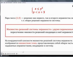
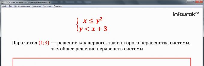
The video lesson begins by introducing the topic and considering an example of finding solutions to a system consisting of inequalities x<=y 2 и у<х+3. Примером точки, координаты которой удовлетворяют условиям обеих неравенств, является (1;3). Отмечается, что, так как данная пара значений является решением обоих неравенств, то она является одним из множества решений. А все множество решений будет охватывать пересечение множеств, которые являются решениями каждого из неравенств. Данный вывод выделен в рамку для запоминания и указания на его важность. Далее указывается, что множество решений на координатной плоскости представляет собой множество точек, которые являются общими для множеств, представляющих решения каждого из неравенств.

Understanding of the conclusions drawn about solving a system of inequalities is strengthened by considering examples. The solution to the system of inequalities x 2 + y 2 is considered first<=9 и x+y>=2. Obviously, solutions to the first inequality on the coordinate plane include the circle x 2 + y 2 = 9 and the region inside it. This area in the figure is filled with horizontal shading. The set of solutions to the inequality x+y>=2 includes the line x+y=2 and the half-plane located above. This area is also indicated on the plane by strokes in a different direction. Now we can determine the intersection of two solution sets in the figure. It is contained in a circle segment x 2 + y 2<=9, который покрыт штриховкой полуплоскости x+y>=2.
Next, we analyze the solution to the system of linear inequalities y>=x-3 and y>=-2x+4. In the figure, next to the task condition, a coordinate plane is constructed. A straight line is constructed on it, corresponding to the solutions of the equation y=x-3. The solution area for the inequality y>=x-3 will be the area located above this line. She is shaded. The set of solutions to the second inequality is located above the line y=-2x+4. This straight line is also constructed on the same coordinate plane and the solution area is hatched. The intersection of two sets is the angle constructed by two straight lines, together with its interior region. The solution area of the system of inequalities is filled with double shading.

When considering the third example, the case is described when the graphs of the equations corresponding to the inequalities of the system are parallel lines. It is necessary to solve the system of inequalities y<=3x+1 и y>=3x-2. A straight line is constructed on the coordinate plane corresponding to the equation y=3x+1. Range of values corresponding to solutions of the inequality y<=3x+1, лежит ниже данной прямой. Множество решений второго неравенства лежит выше прямой y=3x-2. При построении отмечается, что данные прямые параллельны. Область, являющаяся пересечением двух множеств решений, представляет собой полосу между данными прямыми.

The video lesson “Systems of Inequalities with Two Variables” can be used as a visual aid in a lesson at school or replace the teacher’s explanation when studying the material on your own. A detailed, understandable explanation of solving systems of inequalities on the coordinate plane can help present material during distance learning.
, and even more so systems of inequalities with two variables, it seems quite a difficult task. However, there is a simple algorithm that helps solve seemingly very complex problems of this kind easily and without much effort. Let's try to figure it out.
Let us have an inequality with two variables of one of the following types:
y > f(x); y ≥ f(x); y< f(x); y ≤ f(x).
To depict the set of solutions to such an inequality on the coordinate plane, proceed as follows:
- We build a graph of the function y = f(x), which divides the plane into two regions.
- We select any of the resulting areas and consider an arbitrary point in it. We check the feasibility of the original inequality for this point. If the test results in a correct numerical inequality, then we conclude that the original inequality is satisfied in the entire region to which the selected point belongs. Thus, the set of solutions to the inequality is the region to which the selected point belongs. If the result of the check is an incorrect numerical inequality, then the set of solutions to the inequality will be the second region to which the selected point does not belong.
- If the inequality is strict, then the boundaries of the region, that is, the points of the graph of the function y = f(x), are not included in the set of solutions and the boundary is depicted with a dotted line. If the inequality is not strict, then the boundaries of the region, that is, the points of the graph of the function y = f(x), are included in the set of solutions to this inequality and the boundary in this case is depicted as a solid line. Now let's look at several problems on this topic.
Task 1.
What set of points is given by the inequality x · y ≤ 4?
Solution.
1) We build a graph of the equation x · y = 4. To do this, we first transform it. Obviously, x in this case does not turn to 0, since otherwise we would have 0 · y = 4, which is incorrect. This means we can divide our equation by x. We get: y = 4/x. The graph of this function is a hyperbola. It divides the entire plane into two regions: the one between the two branches of the hyperbola and the one outside them.
2) Let’s select an arbitrary point from the first region, let it be point (4; 2). Let's check the inequality: 4 · 2 ≤ 4 – false.
This means that the points of this region do not satisfy the original inequality. Then we can conclude that the set of solutions to the inequality will be the second region to which the selected point does not belong.
3) Since the inequality is not strict, we draw the boundary points, that is, the points of the graph of the function y=4/x, with a solid line.
Let us paint the set of points that defines the original inequality in yellow (Fig. 1).
Task 2.
Draw the area defined on the coordinate plane by the system
Solution.
To begin with, we build graphs of the following functions (Fig. 2):
y = x 2 + 2 – parabola,
y + x = 1 – straight line
x 2 + y 2 = 9 – circle.

Now let's look at each inequality separately.
1) y > x 2 + 2.
We take the point (0; 5), which lies above the graph of the function. Let's check the inequality: 5 > 0 2 + 2 – true.
Consequently, all points lying above the given parabola y = x 2 + 2 satisfy the first inequality of the system. Let's paint them yellow.
2) y + x > 1.
We take the point (0; 3), which lies above the graph of the function. Let's check the inequality: 3 + 0 > 1 – true.
Consequently, all points lying above the straight line y + x = 1 satisfy the second inequality of the system. Let's paint them with green shading.
3) x 2 + y 2 ≤ 9.
We take the point (0; -4), which lies outside the circle x 2 + y 2 = 9. We check the inequality: 0 2 + (-4) 2 ≤ 9 – incorrect.
Consequently, all points lying outside the circle x 2 + y 2 = 9 do not satisfy the third inequality of the system. Then we can conclude that all points lying inside the circle x 2 + y 2 = 9 satisfy the third inequality of the system. Let's paint them with purple shading.

Do not forget that if the inequality is strict, then the corresponding boundary line should be drawn with a dotted line. We get the following picture (Fig. 3).

The search area is the area where all three colored areas intersect with each other (Fig. 4).
Questions for notes

Write an inequality whose solution is a circle and points inside the circle: 
Find the points that solve the inequality:
1) (6;10)
2) (-12;0)
3) (8;9)
4) (9;7)
5) (-12;12)
It is often necessary to depict on the coordinate plane a set of solutions to an inequality with two variables. A solution to an inequality in two variables is a pair of values of these variables that turns the inequality into a true numerical inequality.
2у+ Zx< 6.
First, let's construct a straight line. To do this, we write the inequality in the form of the equation 2у+ Zx = 6 and express y. Thus, we get: y=(6-3x)/2.
This line divides the set of all points of the coordinate plane into points located above it and points located below it.
Take a meme from each area control point, for example A (1;1) and B (1;3)
The coordinates of point A satisfy this inequality 2y + 3x< 6, т. е. 2 . 1 + 3 . 1 < 6.
Coordinates of point B Not satisfy this inequality 2∙3 + 3∙1< 6.
Since this inequality can change sign on the straight line 2y + 3x = 6, then the inequality is satisfied by the set of points in the region where point A is located. Let us shade this region.
Thus, we have depicted the set of solutions to the inequality 2y + 3x< 6.
Example
Let us depict the set of solutions to the inequality x 2 + 2x + y 2 - 4y + 1 > 0 on the coordinate plane.
Let's first build a graph of the equation x 2 + 2x + y 2 - 4y + 1 = 0. Let's separate the equation of the circle in this equation: (x 2 + 2x + 1) + (y 2 - 4y + 4) = 4, or (x + 1) 2 + (y - 2) 2 = 2 2 .
This is the equation of a circle with a center at point 0 (-1; 2) and radius R = 2. Let's construct this circle.

Since this inequality is strict and the points lying on the circle itself do not satisfy the inequality, we construct the circle with a dotted line.
It is easy to check that the coordinates of the center O of the circle do not satisfy this inequality. The expression x 2 + 2x + y 2 - 4y + 1 changes its sign on the constructed circle. Then the inequality is satisfied by points located outside the circle. These points are shaded.
Example
Let us depict on the coordinate plane the set of solutions to the inequality
(y - x 2)(y - x - 3)< 0.
First, let's build a graph of the equation (y - x 2)(y - x - 3) = 0. It is a parabola y = x 2 and a straight line y = x + 3. Let's build these lines and note that changing the sign of the expression (y - x 2)(y - x - 3) occurs only on these lines. For point A (0; 5), we determine the sign of this expression: (5- 3) > 0 (i.e., this inequality does not hold). Now it is easy to mark the set of points for which this inequality is satisfied (these areas are shaded).

Algorithm for solving inequalities with two variables
1. Let us reduce the inequality to the form f (x; y)< 0 (f (х; у) >0; f (x; y) ≤ 0; f (x; y) ≥ 0;)
2. Write the equality f (x; y) = 0
3. Recognize the graphs written on the left side.
4. We build these graphs. If the inequality is strict (f (x; y)< 0 или f (х; у) >0), then - with dashes, if the inequality is not strict (f (x; y) ≤ 0 or f (x; y) ≥ 0), then - with a solid line.
5. Determine how many parts of the graphics the coordinate plane is divided into
6. Select a control point in one of these parts. Determine the sign of the expression f (x; y)
7. We place signs in other parts of the plane, taking into account alternation (as using the interval method)
8. We select the parts we need in accordance with the sign of the inequality we are solving and apply shading
Subject: Equations and inequalities. Systems of equations and inequalities
Lesson:Equations and inequalities with two variables
Let us consider in general terms an equation and an inequality with two variables.
Equation with two variables;
Inequality with two variables, the inequality sign can be anything;
Here x and y are variables, p is an expression that depends on them
A pair of numbers () is called a partial solution of such an equation or inequality if, when substituting this pair into the expression, we obtain the correct equation or inequality, respectively.
The task is to find or depict on a plane the set of all solutions. You can rephrase this task - find the locus of points (GLP), construct a graph of an equation or inequality.
Example 1 - solve equation and inequality:
In other words, the task involves finding the GMT.
Let's consider the solution to the equation. In this case, the value of the variable x can be any, so we have:
Obviously, the solution to the equation is the set of points forming a straight line

Rice. 1. Equation Graph Example 1
The solutions to a given equation are, in particular, the points (-1; 0), (0; 1), (x 0, x 0 +1)
The solution to the given inequality is a half-plane located above the line, including the line itself (see Figure 1). Indeed, if we take any point x 0 on the line, then we have the equality . If we take a point in a half-plane above a line, we have . If we take a point in the half-plane under the line, then it will not satisfy our inequality: .
Now consider the problem with a circle and a circle.
Example 2 - solve equation and inequality:
We know that the given equation is the equation of a circle with center at the origin and radius 1.

Rice. 2. Illustration for example 2
At an arbitrary point x 0, the equation has two solutions: (x 0; y 0) and (x 0; -y 0).
The solution to a given inequality is a set of points located inside the circle, not taking into account the circle itself (see Figure 2).
Let's consider an equation with modules.
Example 3 - solve the equation:
In this case, it would be possible to expand the modules, but we will consider the specifics of the equation. It is easy to see that the graph of this equation is symmetrical about both axes. Then if the point (x 0 ; y 0) is a solution, then the point (x 0 ; -y 0) is also a solution, the points (-x 0 ; y 0) and (-x 0 ; -y 0) are also a solution .
Thus, it is enough to find a solution where both variables are non-negative and take symmetry about the axes:

Rice. 3. Illustration for example 3
So, as we see, the solution to the equation is a square.
Let's look at the so-called area method using a specific example.
Example 4 - depict the set of solutions to the inequality:
According to the method of domains, first of all we consider the function on the left side if there is zero on the right. This is a function of two variables:
![]()
Similar to the method of intervals, we temporarily move away from the inequality and study the features and properties of the composed function.
ODZ: that means the x axis is being punctured.
Now we indicate that the function is equal to zero when the numerator of the fraction is equal to zero, we have:
We build a graph of the function.

Rice. 4. Graph of the function, taking into account the ODZ
Now consider the areas of constant sign of the function; they are formed by a straight line and a broken line. inside the broken line there is area D 1. Between a segment of a broken line and a straight line - area D 2, below the line - area D 3, between a segment of a broken line and a straight line - area D 4
In each of the selected areas, the function retains its sign, which means it is enough to check an arbitrary test point in each area.
In the area we take the point (0;1). We have:
![]()
In the area we take the point (10;1). We have:
![]()
Thus, the entire region is negative and does not satisfy the given inequality.
In the area, take the point (0;-5). We have:
![]()
Thus, the entire region is positive and satisfies the given inequality.