Sections:
GOAL: learn to determine absolute and relative heights from maps, build relief profiles.
- consolidate the concepts of “relief”, “mid-ocean ridge”, “ocean bed”, “deep-sea trench”, “island”, “mountains”, “plains”;
- build a profile of the ocean floor relief and a land relief profile using a physical map;
- continue to develop the ability to compile characteristics of a geographical object;
- check the level of mastery of basic concepts and definitions.
PROGRESS
I. Teacher's opening speech.
A terrain profile is a drawing depicting a section of terrain with a vertical plane, and the direction on the map along which the profile is constructed is profile line.
The order of practical work:
- Draw a profile line.
- Prepare the basis for building a profile. Select horizontal and vertical scale.(horizontal scale, as a rule, is taken to be equal to the map scale, vertical scale – depending on the height, depth of a geographical feature, the elevation between the highest and lowest points). In order to clearly show the nature of the irregularities vertical scale
- is accepted larger (1 cm – 1 km).
- If the scale is very small, the profile line becomes smoothed, as a result of which visibility is lost.
- A sheet of paper is applied with the bottom or top edge to the profile line and from each intersection of it with the horizontal, a perpendicular is drawn to the line that corresponds to the mark of this horizontal.
At the intersection of vertical lines with the corresponding horizontal lines on the plan, place points on the base. The intersection points of these lines with the elevation lines are connected by hand with a smooth curve and we obtain a profile of the relief of the earth's surface.
- II. Practical task 1.
- (done by students under the guidance of a teacher using a PowerPoint presentation with animation)
- Construct a profile of the Indian Ocean along the equator using a depth scale.
| Analyze changes in ocean depths along the equator. | Compare data on changes in ocean depths and determine the location of ocean ridges, continental shallows, and continental slope. | ZONE | |
| 1 | CHANGE IN LONGITUDE (Eastern) | 0-200 | AVERAGE DEPTH, m |
| 2 | 42-43° | 2000-4000 | light |
| 3 | 43-45° | 4000-6000 | light blue |
| 4 | 45-65° | 2000-4000 | light |
| 5 | blue | 4000-6000 | light blue |
| 6 | 65-75° | 2000-4000 | light |
| 7 | 75-89° | 4000-6000 | light blue |
| 8 | 89-91° | 2000-4000 | light |
| 9 | 91-97° | 0-200 | AVERAGE DEPTH, m |
As a result of analyzing the table data, students establish that 1, 9 are shelf zones, 3, 5, 7 are zones of greatest depth, 4, 6 are zones of oceanic ridges. Students should pay attention to the sharp change in depths during the transition from the 1st to the 2nd and from the 8th to the 9th zones and once again explain the concepts of “continental slope” and “ocean bed”.
III. Practice 2 (done by students with partial help from the teacher). The work is done on the interactive whiteboard and in student notebooks.

- Construct a profile of South America along the equator using an altitude scale.
- Conduct an analysis of changes in continental heights along the equator.
- Compare data on changes in the heights of the continent and determine the location of mountains, hills and lowlands.
| Analyze changes in ocean depths along the equator. | CHANGE IN LONGITUDE (Western) | AVERAGE HEIGHT, m | COLOR ON THE PHYSICAL MAP OF THE HEMISPHERES |
| 1 | 79-81° | 0-200 | green |
| 2 | 78-79° | 200-500 | yellow |
| 3 | 76- 78° | 500-5000 | brown |
| 4 | 69-76° | 200-500 | yellow |
| 5 | 61-69° | 0-200 | green |
| 6 | 58-61° | 200-500 | yellow |
| 7 | 56-58° | 0-200 | green |
| 8 | 53-56° | 200-500 | yellow |
| 9 | 51-53° | 0-200 | green |
IV. Analysis of the work done and conclusion:
constructing a terrain profile helps to better imagine the variety of relief forms and, consequently, the influence of the terrain on its climatic features, on the distribution of flora and fauna (PowerPoint presentation with animation “The influence of relief on the distribution of precipitation”)
Literature:
- Atlas. Planet Earth – 6th grade M., Education 2003
- E.Yu.Mishnyaeva, O.G. Kotlyar Planet Earth – 6th grade workbook M., Prosveshchenie 2007
- V.I.Sirotin “Practical work in geography, grades 6-10 M., ARCTI-ILEKSA 1998
To use presentation previews, create a Google account and log in to it: https://accounts.google.com
Slide captions:
Constructing a terrain profile To help prepare for the Unified State Exam
Construct a profile of the terrain along line A - B. To do this, transfer the basis for constructing the profile to answer form No. 2, using a horizontal scale of 1 cm 50 m and a vertical scale of 1 cm 5 m. Indicate the position of the spring on the profile with an “X” sign.
We attached the edge of a sheet of paper to the line connecting the given points, marked with lines the horizontal lines through which our direction passes, signing their marks. 155 m 150 m 145 m 150 m 145 m
1. Attach it to the horizontal line where you will build the profile. Since our scale is 2 times larger, we will lay out the horizontal distance between two adjacent verticals 2 times larger. 2. Restore the perpendiculars until they intersect with the corresponding horizontal lines. These intersections will give a series of points; they are connected by a smooth curve, which will express the profile of the terrain. 3. Two points have the same elevation marks, and between them lies a negative relief form (in our case, a spring), then the line connecting points with the same height should be concave. 155 150 145 145 150 145
1) In the figure in the answer, the length of the horizontal line of the profile base is 80 ± 2 mm, and the distance from the left vertical axis to the spring is 29 ± 2 mm. 2) The profile shape basically coincides with the standard. 3) At site 1 the slope is steeper than at site 2 The answer includes all three elements named above - 2 points The answer includes one (1st) OR two (any) of the above elements - 1 point All answers that do not meet the above criteria grading 1 and 2 points - 0 points
Profile– a reduced image of a vertical section of a section of the earth’s surface. The construction of a longitudinal profile AB on graph paper is carried out in the following order:
Line AB is drawn on the plan, a distance of 1 cm is set aside on both sides of it and a rectangular section is demarcated (Fig. 6.5.);
In the lower half of the graph paper, a profile is drawn along the length of a given line AB, and its name is signed to the left of each column (Fig. 6.6.);
Rice. 6.5 Terrain plan on the line of constructing the longitudinal profile
(according to Neumyvakin, 1985).
Using a meter, draw the outlines of the situation from a map or plan in the “Terrain Plan” column and draw the drawn objects with the corresponding symbols;
On the plan, the points of intersection of the profile line with the horizontal lines and characteristic points of inflections of the terrain are marked, numbered in order;
The profile indicates the vertical and horizontal scales of its construction. On a horizontal scale, the distances between the marked points are laid out using a measuring solution (column “Distances”), on a vertical scale – the marks of points on perpendiculars. The vertical scale is usually 10 times larger than the horizontal one.
Using a measuring solution, transfer the distances between the marked points to the “Distances” column, at the same time, using a scale bar, determine the values of these distances and write them down in the corresponding intervals of this column;
Using the signatures of the contour lines, the elevation marks of the points of their intersection with the profile line are determined, the height marks of the characteristic points are determined by interpolation, rounded to 0.1 m, the resulting values are recorded in the “elevation marks” column;
For the top drawing line, taken as a conditional level surface, a conditional height value is selected so that the drawing is compact. On the perpendiculars to the top line of the graph, the height values are laid down, reduced by the height of the conditional level surface. The ends of the segments are connected by straight lines and the terrain profile of section AB is obtained.
Calculate the slopes between the profile points and write down their values in thousandths of a unit (for example, 6 or 0.006). The directions of the slopes are shown by conventional lines, which are drawn at appropriate intervals from the upper corner to the lower (for a negative slope), and from the bottom to the upper (for a positive slope).

Rice. 6.6. Longitudinal profile along line AB,
Slope scale – is a nomogram for determining slopes from a map or plan, constructed as follows. The horizontal distance is determined for various values of i (for example, 0.02, 0.04, 0.06, etc.) using the formula:
Then they are laid on the corresponding perpendiculars to a straight line, at equal, arbitrary intervals. The ends of the perpendiculars are connected by a smooth curve.
Layout scale – n is a nomogram for determining inclination angles from a map or plan, constructed as follows. The horizontal distance for various inclination angles (for example, 1°, 2°, 3°, etc.) is determined by the formula:
Then they are laid on the corresponding perpendiculars to a straight line, at equal, arbitrary intervals. The ends of the perpendiculars are connected by straight lines.
Exercise
1. Using a topographic map, determine the marks of points, calculate the slopes of lines, and determine their elevations.
2. Construct a longitudinal profile using a topographic map.
Work order
Exercise 1. Using the topographic map obtained in work No. 4, determine the heights of all the vertices of the polygon and calculate the values of the slopes on the sides of the polygon.
Task 2. On graph paper, draw a longitudinal profile along the line indicated on the topographic map obtained in work No. 4.
Determination of the area of the site.
Goal of the work: learn to calculate land areas on a map in various ways.
General information
Analytical method– areas are determined from the results of measurements of lines and angles on the ground or from the coordinates of polygon points using formulas of geometry, trigonometry and analytical geometry.
The general formula for finding the area of any n-gon is:
![]()
From this formula, a large number of other formulas are obtained that express the area of a polygon through increments of coordinates and coordinates of vertices, for example:
![]()
Since here both sides of the equality represent the sum of the product of the abscissa of each point and the ordinate of the same point. Then we get:
![]()
Now let's make a replacement:
![]()
Because both sides of this equality represent the sum of the products of the abscissa of each point and the ordinate of the subsequent point. Then the expression will take the form:
that is, the doubled area of the polygon is equal to the sum of the products of each ordinate and the difference between the abscissas of the previous and subsequent points.
The following expression is obtained similarly:
![]()
Calculation control is carried out according to the formulas:

Here are other formulas for finding the area of a polygon through increments of coordinates and coordinates of vertices without derivation:

Graphic method– areas are determined based on the results of measuring lines on a map or plan, when the area shown on the plan (or map) is first divided into simple geometric shapes, triangles, rectangles and trapezoids (Fig. 7.1). The sum of the areas of geometric figures gives the area of the site. The geometric method also includes calculating area using palettes.

Rice. 7.1. Geometric figures and their elements.
Formulas for calculating the area of a triangle (Fig. 7.1. a):

Formulas for calculating the area of a trapezoid (Fig. 7.1. b):
Formulas for calculating the area of a quadrilateral (Fig. 7.1.c, c)
Palette - is a sheet of glass, celluloid, tracing paper or other transparent material, drawn with thin lines into squares (square palette) or parallel straight lines (parallel palette).
A square palette is a network of mutually perpendicular lines drawn every 1 or 2 mm. The area is determined by counting the cells of the palette superimposed on the figure; the proportions of cells dissected by the contour are taken into account by eye. Knowing the area of one square, which depends on the scale of the plan, the area of the entire figure is determined by the formula:
![]()
where, s is the area of one square, on the plan scale;
n – the number of whole squares that fit into the determined area;
m – the number of squares determined from their parts cut by a contour.
To simplify the calculations, thickened lines are drawn every 0.5 or 1 cm so that the number of cells can be counted in groups. To control, the area of this area is measured again, turning the palette 45°.
Parallel palette - a series of parallel lines drawn predominantly at 2 mm intervals (from 2 to 5 mm). The contour area of this palette is calculated as follows. Place it on the plan so that the extreme points of the contour of section 1 and 16 are in the middle between the lines of the palette (Fig. 7.2.) As a result, the section is divided into separate trapezoids with a height h and middle lines s 2-3, s 4-5, ..., s 14-15, which are measured on the plan scale (the bases of the trapezoid are shown with a dotted line). Since the area of each trapezoid is equal to the product s i ×h, the total area of the site will be:

Rice. 7.2. Determining the contour area with a parallel palette.
The sum of distances Σs i is sequentially collected into the meter solution: taking the distance s 2-3, move the left needle of the meter to point 5, and the right one is set to continue the line 4-5 at point k, after which the meter solution is increased by moving the left needle to point 4. Then the sum of the middle lines (s 2-3 + s 4-5) will be collected in the 4-k meter solution. Further measurements are continued in the same sequence. If, in the process of dialing distances, the meter solution turns out to be larger than the size of the palette along its length AB, then the sum of the middle lines is dialed in parts in several steps. The total length of the measured center lines is determined using a scale bar and multiplied by the height h, corresponding to the number of meters on the plan scale, then the resulting area is converted to hectares.
For control, measure the area at the second position of the palette, turning it 60-90° relative to the original position. The relative error in determining the area with a palette is 1:50 – 1:100. It is recommended to use a square palette when defining a polygon with an area of up to 2 cm2, a parallel palette – up to 10 cm2.
Mechanical method– areas are determined from a plan or map using special instruments – planimeters (Fig. 7.3.).
Planimeter- a mechanical or electronic device that, by tracing a flat figure of any shape, determines its area. Planimeters are divided into linear - in which all points of the device for tracing a figure are movable, and polar - in which one point (pole) is stationary during tracing.
The area of the figure is calculated as follows. Before starting the circuit, index 5 is set at the starting point of the circuit and count n 1 is taken from the counting mechanism. Keeping the index on the contour line, trace the figure clockwise to the starting point and take the count n 2. after tracing The resulting difference in readings Δn= n 2 .– n 1 shows the length of the counting roller path, expressed in planimeter divisions, or otherwise the number of divisions τ corresponding to the area of the circled figure.

Rice. 7.3. Polar planimeter (a) and diagram of its counting mechanism (b)
(according to Maslov, 2006).
1 – hinged connection of levers; 2 – bypass lever; 3 – pole lever; 4 – pole; 5 – bypass index; 6 – support screw (pin); 7 – counting roller; 8 – vernier (vernier); 9 – dial of the counting mechanism.
The counting mechanism consists of four digits (Fig. 22, b). The first digit shows the number of revolutions made to the dial 9; if the pointer is between two digits, then the smaller digit is read. The second digit shows the tenths of a revolution of the counting roller 7 and is read on the counting roller relative to the zero of the vernier 8, the tenths of a revolution of the roller are signed. The third digit shows the hundredths of a revolution, which are read between the tenths of a revolution stroke and the vernier zero. The fourth digit shows thousandths of a revolution, which are read on the vernier by a stroke that coincides with any stroke of the counting roller.
To control changes, the contours are performed at least twice, the permissible differences are no more than 3 divisions for a figure area of up to 200 cm 2 and 4 divisions for - 400 cm 2. If discrepancies are acceptable, then the average is obtained from the two results.
The area of the figure, determined by the contours of the planimeter with the pole installed outside the figure, is calculated using the formula:
where, p is the division price of the planimeter, i.e. area corresponding to one division τ.
![]()
where, R – length of the bypass lever;
M is the denominator of the numerical scale of the plan.
To practically determine the division price p, a figure with a known area is repeatedly traced with a fixed installation of the bypass lever R. As such a figure, 2-3 squares of the coordinate grid are usually taken. To increase the accuracy of measurements, the figure is circled at least four times: twice when the mechanism is positioned on the right (MP) and twice when the mechanism is positioned on the left (ML). The measurement results are entered in a special form (Appendix 4)
When tracing a figure, the following requirements must be met:
1. The plan is laid out, straightened and secured on a flat surface.
2. The pole of the planimeter is installed in such a way that when tracing the figure, the angle between the levers θ is no less than 30° and no more than 150°, and its deviations in both directions from 90° would be approximately the same.
3. The starting point for setting the bypass index is selected on the contour in such a way that when the planimeter moves at the beginning and at the end of the bypass, the counting roller does not rotate at all or its rotation is slow.
Exercise
1. Calculate the area of the polygon based on points with known rectangular coordinates.
2. Calculate the area of the landfill using the topographic map obtained in work No. 4, graphically and mechanically.
Work order
Exercise 1. Calculate the area of the polygon at points with known rectangular coordinates, fill out the sheet based on the calculation results (Table 9). Calculations are carried out according to the starting points in accordance with the task option (Table 10).
Table 7.1
Sheet for calculating the area of a polygon based on its vertices
| Vertex No. | Coordinates, m | |||||
| x i | y i | y i+ 1 – y i- 1 | x i -1 –x +1 | x i (y i+1 – y i-1) | y i (x i-1 –x i+1) | |
Table 7.2.
Test tasks for calculating the area of a polygon analytically.
| Option number | coordinates of starting points | |||||||
| X | U | X | U | X | U | X | U | |
| 6 134 629,3 | 9 416 014,3 | 6 131 421,3 | 9 484 701,6 | 6 131 975,2 | 9 415 881,6 | 6 132 215,2 | 9 413 215,1 | |
| 6 233 952,4 | 9 573 914,8 | 6 133 517,2 | 9 485 025,7 | 6 133 952,4 | 9 413 914,8 | 6 134 629,3 | 9 416 014,3 | |
| 6 163 952,5 | 9 163 914,8 | 6 133 517,2 | 9 485 025,7 | 6 233 517,2 | 9 575 025,7 | 6 233 952,4 | 9 573 914,8 | |
| 6 131 421,3 | 9 514 701,6 | 6 161 421,3 | 9 514 701,6 | 6 133 517,2 | 9 485 025,7 | 6 131 258,4 | 9 484 701,6 | |
| 6 131 975,2 | 9 415 881,6 | 6 133 415,9 | 9 517 608,2 | 6 161 421,3 | 9 514 701,6 | 6 163 952,5 | 9 163 914,8 | |
| 6 133 952,4 | 9 413 914,8 | 6 131 975,2 | 9 415 881,6 | 6 133 415,9 | 9 517 608,2 | 6 131 421,3 | 9 514 701,6 | |
| 6 134 629,3 | 9 416 014,3 | 6 133 952,4 | 9 413 914,8 | 6 131 975,2 | 9 415 881,6 | 6 132 215,2 | 9 413 215,1 | |
| 6 233 952,4 | 9 573 914,8 | 6 233 517,2 | 9 575 025,7 | 6 133 952,4 | 9 413 914,8 | 6 134 629,3 | 9 416 014,3 | |
| 6 163 952,5 | 9 163 914,8 | 6 133 517,2 | 9 485 025,7 | 6 233 517,2 | 9 575 025,7 | 6 233 952,4 | 9 573 914,8 | |
| 6 131 421,3 | 9 514 701,6 | 6 161 421,3 | 9 514 701,6 | 6 133 517,2 | 9 485 025,7 | 6 131 421,3 | 9 484 701,6 | |
| 6 131 975,2 | 9 415 881,6 | 6 133 415,9 | 9 517 608,2 | 6 161 421,3 | 9 514 701,6 | 6 163 952,5 | 9 163 914,8 | |
| 6 133 952,4 | 9 413 914,8 | 6 161 421,3 | 9 547 521,4 | 6 133 415,9 | 9 517 608,2 | 6 131 421,3 | 9 514 701,6 |
Task 2. Calculate the area of the polygon using the topographic map obtained in work No. 4, graphically: dividing it into simple geometric shapes, using square and linear palettes.
Calculate the area of the landfill using the topographic map obtained in work No. 4 mechanically (Appendix 3).
BIBLIOGRAPHY
1. Bakanova V.V. Geodesy: textbook for universities / V.V. Bakanova; under. total ed. L.M. Komarkova; M.: Nedra, 1980, 277 S.
2. Barshay S.E. Engineering geodesy / S.E. Barshai, V.F. Nesterenok, L.S. Khrenov; under general ed. L.S. Khrenova; Minsk: Higher School, 1976, 400С.
3. Dyakov B.N. Geodesy: textbook for universities / B.N. Dyakov; resp. ed. I.V. Lesnykh; SSGA 2nd ed., revised. and additional Novosibirsk: SGGA, 1997, 173 P.
4. Izmailov P.I. Workshop on geodesy / P.I. Izmailov; under. total ed. THEM. Bludova; M.: Nedra, 1970, 376 S.
5. Maslov A.V. Geodesy / A.V. Maslov, A.V. Gordeev, Yu.G. Farm laborers; under general ed. V.A. Churakova; Ed. 6th revision and additional M.: Kolos, 2006, 598С.
6. Mikheeva D.Sh. Engineering geodesy / D.Sh. Mikhelev, M.I. Kiselev, E.B. Klyushin; edited by D.Sh. Mikheleva; 6th ed. erased M.: ed. Center Academy, 2006, 480 S.
7. Neumyvakin Yu.K. Workshop on geodesy / Yu.K. Neumyvakin, A.S. Smirnov; under general ed. N.T. Kuprina; M.: Nedra, 1985, 200 pp.
8. Poklad G.G. Geodesy: textbook for universities / G.G. Poklad, S.P. Gridnev; Voronezh. state agrarian univ., M.: Academic project, 2007, 592С.
9. Peters I. Six-digit tables of trigonometric functions / I. Peters; under. total ed. L.M. Komarkova; M.: Nedra, 1975, 300 S.
10. Instructions for calculating areas: Approved. Ch. Department of Land Use, Land Management and Soil Protection of the Ministry of Agriculture of the RSFSR 04/24/74. M., 1974, 48 S.
11. Conventional signs for topographic plans at scales 1:5 000, 1:2 000, 1:1 000, 1:500: Approved. GUGK under the Council of Migrants of the USSR 11.25.86. M.: Kartgeoizdat - Geoizdat, 2000, 286 pp.
12. Fedotov G.A. Engineering geodesy / G.A. Fedotov; under general ed. L.A. Savina; M.: Higher school, 2002, 463 pp.
13. Chizhmakov A.F. Workshop on geodesy / A.F. Chizhmakov, A.M. Krivochenko, V.M. Lazarev [and others]; under general ed. L.M. Komarkova; M.: Nedra, 1977, 240 S.
14. Yuzhaninov V.S. Cartography with the basics of topography / V.S. Yuzhaninov; under general ed. Yu.E. Ivanova; M.: Higher School, 2001, 302 S.
Annex 1

Appendix 2
 |  |
 |
|
 |
|
 |
Appendix 3
EXERCISE
1. Determination of rectangular and geographical coordinates:
Determine the rectangular coordinates of all the vertices of the polygon (make a schematic drawing showing the position of the points relative to the coordinate axes).
Determine the geographic coordinates of all vertices of the polygon.
Table 1.
Determining the coordinates of the polygon vertices from the map.
2. Orientation of directions:
Measure geographic azimuths and directional angles of all sides of the polygon on the map, calculate the magnetic azimuth. Show all measured and calculated values on a schematic drawing.
Using the measured interior angles of the polygon, taking the directional angle α 1-2 for the original, calculate sequentially the directional angles of all sides of the polygon using the formula for transferring the directional angle. Calculate angles in a clockwise direction.
Using the values of directional angles and azimuths, calculate the directions of the sides
Table 2.
Determining the lengths of the polygon sides and their reference angles from the map
3. Inverse geodetic problem. Using the plan coordinates of the polygon vertices, determine the lengths and directional angles of all sides of the polygon.
Table 3.
Determining the lengths of the polygon sides and their directional angles from the solution
inverse geodetic problem
4. Relief image on a topographic map:
Determine the heights of all vertices of the polygon.
Calculate the slope values on the sides of the polygon.
Construct a longitudinal profile on graph paper along the line indicated in the assignment.
5. Calculation of the area of the polygon:
Using the coordinates of the polygon vertices, calculate the area of the polygon.
Calculate the area of a polygon graphically
Appendix 4
Planimeter No. 4081 R=133.4 p=0.02
| Section No. | Pole position | Samples n 1, n 2 and n 3 | Differences n 1 – n 2 n 2 – n 3 | Average of the differences | Area in divisions of plani-meter | Area, ha | Amendment | Linked area of sections, hectares | Note |
| I | PL | 1590,5 | 31,80 | -0,06 | 31,74 | ||||
| PP | 1589,5 | ||||||||
| II | PL | 33,72 | -0,07 | 33,65 | |||||
| PP | |||||||||
| III | PL | 17,82 | -0,06 | 17,79 | |||||
| PP | |||||||||
Introduction........................................................ ........................................................ ... 3
Calculation and graphic work No. 1................................................... ................. 4
1. Scale. Conventional topographical signs.................................................... 4
1.1 Scale................................................... ......................................... 4
1. 2 Conventional topographic signs.................................................. ...... 9
2. Orientation of directions.................................................... ............... eleven
3. Nomenclature and layout of topographic plans and maps............ 18
Calculation and graphic work No. 2....................................................... 26
4. Determination of geographical and rectangular coordinates of points and reference angles of directions on the map.................................................... ........................................... 26
6. Basic landforms. Problems solved on topographic maps and plans. 33
7. Determination of the area of the site................................................... .............. 40
BIBLIOGRAPHY................................................ ........................ 47
Annex 1................................................ ........................................... 48
Appendix 3................................................... ........................................... 50
Appendix 4................................................... ........................................... 52
The twenty-eighth task of the Unified State Exam in geography involves working with maps and plans of the area. It is necessary to build a terrain profile along straight line AB; on the profile you also need to indicate with a symbol any object shown on the map.
Instructions for building a profile
In order to construct a profile, you need to draw a profile line connecting points A and B, and attach to it the edge of a sheet of paper, on which you need to mark the horizontal lines through which line AB passes. The contour marks need to be signed (the map indicates at what interval they are drawn, the value of one contour is also given, so it is not at all difficult to sign them). This edge of the sheet must be attached to the horizontal line on the form where the profile is being constructed. You need to transfer the marks you made to it like this, drawing perpendiculars to the vertical line in similar values:
After this, the resulting points need to be connected with a smooth curved line. This will be the relief profile. In this task, it is important to take into account the scale: if, for example, according to the map scale, 1 cm is 100 m, and in our drawing, 1 cm should be 50 m, then we will mark the distance between two adjacent verticals twice as large. People are often asked to mark a spring on their profile; as a rule, it is located between two adjacent heights - in this case they need to be connected not by a straight line, but by a concave one.
Analysis of typical options for task No. 28 of the Unified State Exam in geography
First version of the task
Construct a terrain profile along line AB. Transfer the basis for its construction to answer sheet 2, using a horizontal scale of 1 cm = 50 m and a vertical scale of 1 cm = 5 m. Mark the position of the spring with an “X”.

The finished profile for this condition looks something like this:

The length of the horizontal line is approximately 80 mm, the distance from the vertical to the spring is approximately 29 mm. The slope in section 1 should be steeper than in section 2. If all these conditions are met and the shape of the profile is similar to the standard, the student receives 2 points for this task. If the profile is similar to the standard, but the distance and steepness of the slopes do not coincide with the specified parameters, 1 point is given. In other cases, no points are awarded for task 28.
Instructions
Next we move on to a description of urban data. The largest settlements, approximate population, socio-economic buildings (factories, mining sites, etc.) are listed. The most important social buildings (theatres, museums, monuments of regional or regional significance) are also indicated.
note
Before starting to describe any area, you need to indicate the alphanumeric code of the map, the territory it represents, its nature and the purposes for which it is used.
Sources:
- Topographic training of the commander
Geodesy (from the Greek geo - earth and daio - divide) is a science that deals with determining the shape and size of the Earth, measuring objects located on its surface to draw up plans and maps. It is closely related to such natural sciences as geophysics, astronomy and hydrography.

Without geodesy, you will not be able to determine the boundaries of objects according to the given ones. Such, for example, as land plots issued for private ownership. Now that the boundaries of land plots in documents are indicated in a certain coordinate system, it is simply impossible to do without surveyors when registering them. Only they can bring these boundaries into reality.
If you are going to develop and build a house, after the boundaries have been determined, you will need to draw up a detailed site plan. You will receive it by ordering a geodetic survey. The scale of the plan is usually 1:500, it should be so detailed that all the characteristic features of the area and