) A = ||a ik||n 1 by subtracting the value λ from the diagonal elements. This determinant is a polynomial with respect to X - a characteristic polynomial. When opened, X. u. is written like this:
Where S 1 = a 11 + a 22 +... ann- so-called matrix trace, S 2- the sum of all major minors of the 2nd order, i.e. minors of the form i k), etc., and S n- matrix determinant A. Roots of H. u. λ 1 , λ 2 ,..., λ n are called the eigenvalues of the matrix A. For a real symmetric matrix, as well as for a Hermitian matrix, all λ k are real, a real skew-symmetric matrix has all λ k purely imaginary numbers; in the case of a real orthogonal matrix, as well as a unitary matrix, all |λ k| = 1.
H.u. found in a wide variety of areas of mathematics, mechanics, physics, and technology. In astronomy, when determining the secular perturbations of the planets, they also come to chemical equations; hence the second name for X. u. - an age-old equation.
2) H. u. linear differential equation with constant coefficients
a 0λ y (n) + a 1 y (n-1) +... + a n-1 y" + a n y = 0
Algebraic equation that is obtained from a given differential equation after changing the function at and its derivatives by the corresponding powers of λ, i.e. the equation
a 0λ n + a 1λ n-1 + ... + a n-1 y" + a n y = 0.
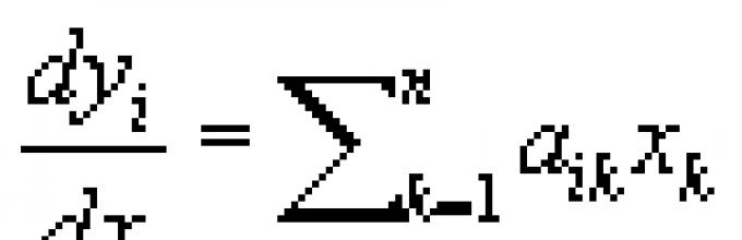
This equation is arrived at by finding a particular solution of the form at = se λ X for a given differential equation. For a system of linear differential equations
![]()
H.u. written using a determinant

H.u. matrices A =
Great Soviet Encyclopedia. - M.: Soviet Encyclopedia. 1969-1978 .
See what a “Characteristic Equation” is in other dictionaries:
In many cases, physical processes occurring in systems are described by a system of ordinary linear differential equations with constant coefficients, which in a fairly general case can be reduced to the differential equation ... Encyclopedia of technology
An algebraic equation of the form: The determinant in this formula is obtained from the determinant of the matrix by subtracting the value x from the diagonal elements; it represents a polynomial in x and is called a characteristic polynomial... Big Encyclopedic Dictionary
characteristic equation- - [V.A. Semenov. English-Russian dictionary of relay protection] Topics relay protection EN characteristic equation ... Technical Translator's Guide
Algebraic equation of the form. The determinant in this formula is obtained from the determinant of the matrix x of diagonal elements; it is a polynomial in x and is called a characteristic polynomial. * * * CHARACTERISTIC… … Encyclopedic Dictionary
characteristic equation- būdingoji lygtis statusas T sritis automatika atitikmenys: engl. characteristic equation; performance equation vok. charakteristische Gleichung, f; Stammgleichung, f rus. characteristic equation, n pranc. équation caractéristique, f … Automatikos terminų žodynas
characteristic equation- būdingoji lygtis statusas T sritis fizika atitikmenys: engl. characteristic equation; performance equation vok. Charakteristische Gleichung, f rus. characteristic equation, n pranc. équation caractéristique, f … Fizikos terminų žodynas
characteristic equation Encyclopedia "Aviation"
characteristic equation- characteristic equation. In many cases, physical processes occurring in systems are described by a system of ordinary linear differential equations with constant coefficients, which in a fairly general case can be reduced... Encyclopedia "Aviation"
Secular equation, see Art. Characteristic polynomial... Mathematical Encyclopedia
A characteristic polynomial is a polynomial that determines the eigenvalues of a matrix. Another meaning: The characteristic polynomial of a linear recurrent is a polynomial. Contents 1 Definition ... Wikipedia
Books
- Characteristic Lie rings and nonlinear integrable equations, Zhiber A.V.. The book is devoted to a systematic presentation of the algebraic approach to the study of nonlinear integrable partial differential equations and their discrete analogues, based on the concept...
The free mode of the circuit does not depend on energy sources, it is determined only by the structure of the circuit and the parameters of its elements. It follows from this that the roots of the characteristic equation p1, p2,..., pn will be the same for all variable functions (currents and voltages).
The characteristic equation can be constructed using various methods. The first method is classical, when the characteristic equation is compiled strictly in accordance with the differential equation according to the classical scheme. When calculating transient processes in a complex circuit, a system of “m” differential equations is compiled according to Kirchhoff’s laws for the circuit diagram after switching. Since the roots of the characteristic equation are common to all variables, the solution of the system of differential equations is performed with respect to any variable (optional). As a result of the solution, an inhomogeneous differential equation with one variable is obtained. Compose a characteristic equation in accordance with the resulting differential equation and determine its roots.
Example. Draw up a characteristic equation and determine its roots for the variables in the diagram in Fig. 59.1. The parameters of the elements are specified in a general form.
System of differential equations according to Kirchhoff's laws:

Let us solve the system of equations for the variable i3, as a result we obtain a non-homogeneous differential equation:

The second way to compile a characteristic equation is to equate to zero the main determinant of the Kirchhoff system of equations for the free component variables.
Let the free component of an arbitrary current have the form iksv = Аkept, then:

The system of equations for the free components is obtained from the Kirchhoff system of differential equations by replacing the derivatives of the variables by the factor p, and the integrals by 1/p. For the example under consideration, the system of equations for free components has the form:

Characteristic equation and its root:

The third way to compile a characteristic equation (engineering) is to equate the input operator resistance of the circuit to zero relative to any of its branches.
The operator resistance of an element is obtained from its complex resistance by simply replacing the factor jω with p, therefore
For the example in question:

The third method is the simplest and most economical, therefore it is most often used when calculating transient processes in electrical circuits.
The roots of the characteristic equation characterize the free transient process in a circuit without energy sources. This process occurs with energy losses and therefore decays over time. It follows from this that the roots of the characteristic equation must be negative or have a negative real part.
In the general case, the order of the differential equation that describes the transient process in the circuit, and, consequently, the degree of the characteristic equation and the number of its roots are equal to the number of independent initial conditions, or the number of independent energy storage devices (coils L and capacitors C). If the circuit diagram contains parallel-connected capacitors C1, C2,... or series-connected coils L1, L2,..., then when calculating transient processes they must be replaced by one equivalent element SE = C1 + C2+... or LE = L1 + L2+...
Thus, the general form of the solution for any variable when calculating the transient process can be compiled only from an analysis of the circuit diagram, without compiling and solving a system of differential equations.
For the example discussed above.
The characteristic equation is compiled for the circuit after switching. It can be obtained in the following ways:
- directly based on a differential equation of the form (2) (see lecture No. 24), i.e. by excluding from the system of equations describing the electromagnetic state of the circuit based on Kirchhoff’s first and second laws, all unknown quantities except one, in relation to which equation (2) is written;
- by using an expression for the input impedance of a sinusoidal current circuit;
- based on the expression of the main determinant.
According to the first method, in the previous lecture, a differential equation was obtained regarding the voltage on the capacitor for a series R-L-C circuit, on the basis of which the characteristic equation is written.
It should be noted that, since the linear circuit is covered by a single transient process, the roots of the characteristic equation are common to all free components of voltages and currents of the circuit branches, the parameters of which are included in the characteristic equation. Therefore, according to the first method of composing a characteristic equation, any variable can be chosen as the variable with respect to which it is written.

Let us consider the application of the second and third methods of composing the characteristic equation using the example of the circuit in Fig. 1.
The composition of the characteristic equation using the input resistance method is as follows:
the input resistance of the AC circuit is recorded;
jw is replaced by operator p;
the resulting expression is equal to zero.
Equation
coincides with the characteristic one.
It should be emphasized that the input resistance can be written relative to the break point of any branch of the circuit. In this case, the active two-terminal network is replaced by a passive one by analogy with the equivalent generator method. This method of composing the characteristic equation assumes the absence of magnetically coupled branches in the circuit; if there are any, it is necessary to carry out their preliminary untying.
For the circuit in Fig. 1 relative to source terminals
 .
.
Replacing jw with p and equating the resulting expression to zero, we write
| . | (1) |
When compiling a characteristic equation based on the expression of the main determinant, the number of algebraic equations on the basis of which it is written is equal to the number of unknown free current components. Algebraization of the original system of integro-differential equations, compiled, for example, on the basis of Kirchhoff's laws or the method of contour currents, is carried out by replacing the symbols of differentiation and integration, respectively, with multiplication and division by the operator p. The characteristic equation is obtained by equating the written determinant to zero. Since the expression for the main determinant does not depend on the right-hand sides of the system of inhomogeneous equations, it can be compiled on the basis of a system of equations written for total currents.
For the circuit in Fig. 1 algebraized system of equations based on the loop current method has the form

Hence the expression for the main determinant of this system
Equating D to zero, we obtain a result similar to (1).
General methodology for calculating transient processes using the classical method
In general, the methodology for calculating transient processes using the classical method includes the following steps:
Examples of calculating transient processes using the classical method
1. Transient processes in the R-L circuit when it is connected to a voltage source

Such processes take place, for example, when connecting electromagnets, transformers, electric motors, etc. to a power source.
Let's consider two cases:
According to the considered method for the current in the circuit in Fig. 2 can be written
Characteristic equation
hence the time constant ![]() .
.
Thus,
| . | (5) |
Substituting (4) and (5) into relation (3), we write
 .
.
In accordance with the first law of commutation. Then
![]() ,
,
Thus, the current in the circuit during the transient process is described by the equation
 ,
,

and the voltage across the inductor is given by
 .
.
The qualitative appearance of the curves and corresponding to the obtained solutions is presented in Fig. 3.
For the second type of source, the forced component is calculated using the symbolic method:
 ,
,
The expression of the free component does not depend on the type of voltage source. Hence,
![]() .
.
Since then
Thus, we finally get
| . | (6) |
Analysis of the resulting expression (6) shows:
If it is significant in magnitude, then over half a period the free component does not decrease significantly. In this case, the maximum value of the transient current can significantly exceed the amplitude of the steady-state current. As can be seen from Fig. 4, where
![]() , the maximum current occurs after approximately . In the limit at .
, the maximum current occurs after approximately . In the limit at .
Thus, for a linear circuit, the maximum value of the transient current cannot exceed twice the amplitude of the forced current: .
Similarly for a linear circuit with a capacitor: if at the moment of switching the forced voltage is equal to its amplitude value and the time constant of the circuit is sufficiently large, then after about half a period the voltage on the capacitor reaches its maximum value, which cannot exceed twice the amplitude of the forced voltage: ![]() .
.
2. Transient processes when disconnecting the inductor from the power source
When the key is opened in the circuit in Fig. 5 forced component of the current through the inductor.
Characteristic equation
![]() ,
,
where ![]() And
And ![]() .
.
According to the first law of commutation
 .
.
Thus, the expression for the transient current is
and voltage across the inductor
 . .
|
(7) |
Analysis (7) shows that when circuits containing inductive elements are opened, large overvoltages can occur, which, without taking special measures, can damage the equipment. Indeed, when ![]() The voltage module on the inductor at the moment of switching will be many times higher than the source voltage: . In the absence of a quenching resistor R, the specified voltage is applied to the opening contacts of the key, as a result of which an arc occurs between them.
The voltage module on the inductor at the moment of switching will be many times higher than the source voltage: . In the absence of a quenching resistor R, the specified voltage is applied to the opening contacts of the key, as a result of which an arc occurs between them.
3. Charging and discharging a capacitor
When the key is moved to position 1 (see Fig. 6), the process of charging the capacitor begins:
![]() .
.
Forced voltage component on a capacitor.
From the characteristic equation
the root is determined ![]() . Hence the time constant.
. Hence the time constant.
The characteristic equation has the form:
To determine the type of free component, it is necessary to draw up and solve the characteristic equation: z(p) = 0. To write the characteristic equation, it is necessary to draw a diagram in which all sources of emf and current should be replaced by their own internal resistance, and the inductance and capacitance resistance should be taken respectively equal Pl and , then it is necessary to break any branch of this circuit, write down its initial resistance relative to the points of break, equate it to zero, solve and determine the roots of p, if the roots turn out to be real negative, then the free component of the desired function:
 ,where m is the number of roots of the equation;
Roots; - permanently integrated.
If the roots of the character equation turn out to be complex conjugate, then the free state will have the form:
 where is the frequency of free vibrations;
The initial phase of free oscillations.
8.Transition time. Determination of practically t pp. Calculation of the transition process time.
The time of the transient process depends on the attenuation coefficient. The inverse value is called the time constant and represents the time during which the value of the free component of the transient process will decrease by e = 2.72 times. The value depends on the circuit and parameters. So for a circuit with a series connection r and L =, and for a series connection
95% completion of the transition process 3.
The easiest way to construct the curves of the free components of the transient process is to set the time t values to 0, ,2.....If there are several real roots, then the resulting curve is obtained by summing the ordinates of the individual terms (Fig. 1.)
Figure 1:

9.10,Transient process in r, C – circuits when connected to a constant voltage source. Perform the analysis using the classical method; give analytical expressions for U C (t); iC(t); graphics. (Classical method).
The equation of state of the rC circuit after switching is as follows:
![]() (1) or rC (2)
(1) or rC (2)
His solution: ![]()
Capacity C after closing the key at t will be charged to a steady value. Free component
Since the initial conditions are zero, according to the commutation law ![]() at t=0, or 0=A, whence A=-E.
at t=0, or 0=A, whence A=-E.
The solution to equation (2) will take the form:
Circuit current i(t)=C
Figure 1.

Figure 2.

Graphs of changes in voltage and current i(t) are shown in Figures 1 and 2. From the figures it can be seen that the voltage on the capacitor increases exponentially from 0 to E, while the current strength at the moment of switching abruptly reaches the value E/r, and then decreases to zero.
11.12.Transient process in r, C – circuits when connected to a sinusoidal voltage source. Perform the analysis using the classical method; give analytical expressions for U C (t); iC(t); graphics. (Classical method).

The equation of state of the rC circuit in the transient mode is as follows
rC ![]() .
.
Solution to this equation:
![]()
Free component
![]() where =rC
where =rC
Since the circuit is linear, then with a sinusoidal effect and in steady state, the voltage on the capacitor will also change according to a sinusoidal law with the frequency of the input effect. Therefore, to determine = we will use the method of complex amplitudes:
![]() ;
; 
![]()
Considering that j= , we get:
Integration constant A of the free component
Let us find from the initial conditions in the circuit taking into account the commutation law:
![]() .At t=0 the last expression has the form
.At t=0 the last expression has the form
Where does A=-
Adding the components and , we obtain the final expression for the voltage across the capacitor in the transient mode:
= + = ![]() - (1)
- (1)
Analysis of expression (1) shows that the transient process in the rC circuit under sinusoidal influence depends on the initial phase of the source emf at the moment of switching and on the time constant of the rC circuit.
If , then =0 and a steady state will occur in the circuit immediately after switching, i.e.
When voltage = - , i.e. The voltage across the capacitor immediately after switching can reach almost double the value of the positive sign, and then gradually approach =.
The phase difference will lead equation (1) to the form:
The difference between this mode and the previous one is that the voltage across the capacitor immediately after switching can reach almost twice the negative value.
For the considered Rc circuit with a sinusoidal current source in steady state, the initial phase of the input voltage does not play any role, but in the transient process its influence is significant.
13.Transient process in r, L, C – circuits when connected to a constant voltage source. Batch process. Analytical expressions for i(t), graphics. (Classical method).
The roots are real, negative, different.
I(t)=I mouth +A1e p 1 t +A2e p 2 t
The process is periodic:
t=0 (i(0)=A1+A2; A1=-A2
{ ![]()
t=0 i l (0)*r+L +Uc(0)=E A1=-A2= ()
i l (t)= ( ![]() )
)
14.Transient process in r, L, C – circuits when connected to a constant voltage source. Critical process. Analytical expressions for i(t), graphics. (Classical method).
i l (t)=i lips +(B1+B2*t)*
t=0: i l (0)=β1=0
![]()
If the roots turn out to be real, negative, equal, then the process is critical.

15.Transient process in r, L, C – circuits when connected to a constant voltage source. Oscillatory process. Analytical expression for i(t), graphics. (Classical method).
P t = -δ±j*ω St ω St =
The roots are negative real, some complex conjugate.
i l (t)=i mouth A1e - δt *sin(ω St t+ψ)

i l (t)=i mouth +(M*cos ω light t+N*sin ω light t)*
i l (t)= * ![]() = *
= *

16. Transient process in r, L, C – circuits when connected to a sinusoidal voltage source. Aperiodic process. Analytical expression for i(t), graphics. (Classical method).
R(t)=E max *sin(ωt+ψ)
2. 
In the classical number of equations in this case is equal to the number of branches of the circuit
The method finds a solution in the form of the sum of a general and a particular solution. The calculation of the transient process is described by a system of ordinary differential equations compiled by one of the calculation methods for instantaneous values of time functions. The solution for each variable of this system is found in the form of the sum of the general and particular solutions. To compile an equation, the following can be used: a method based on the application of Kirchhoff’s laws, the method of nodal potentials, the method of loop currents, etc. For example, a system of differential equations compiled after commutation according to Kirchhoff’s first and second laws has the form:
For example,
The number of equations in this case is equal to the number of branches of the circuit. Let it be necessary to find the current i k in a branch with number K. Eliminating the currents of the branches in sequence, as a result we obtain the current i k and its derivatives up to order n:

The order of the differential equation n is determined by the number of independent reactive elements of the circuit (m). Usually n=m, but depending on the connection method it may be that n Series-connected capacitive elements can be replaced by one element, just as parallel-connected inductive elements can be replaced by one equivalent one. Figure 9.5 shows the replacement of 2 capacitors connected in series with one equivalent one. In general, the order of the differential equation n is equal to: n=n lc -n ce -n lj, where n lc is the number of reactive elements (L and C) in the circuit, n ce is the number of capacitive circuits, n lj is the number of inductive nodes or sections. By capacitive is meant a circuit consisting of capacitive elements or capacitive elements and ideal emf sources, Fig. 9.6.a. By inductive is meant a node into which inductive branches or inductive branches and current sources converge (Fig. 9.6.b), or sections that only inductive branches or inductive branches and current sources cross. Note that the stage of drawing up a differential equation is not mandatory and the transition current or voltage can be found without drawing up an equation. As was indicated, in the classical method of calculating transient processes solving the equations A particular solution describes a regime called forced. The solution of a homogeneous equation (the right side is zero) describes the process in the absence of external EMF and current sources and is called free. Free and forced currents, voltages, and charges are considered accordingly. Thus, the current in the branch with number K is represented as a sum. The characteristic equation is compiled for the circuit after switching. It can be obtained in the following ways: Directly based on a differential equation of the form (1.2), i.e. by excluding from the system of equations describing the electromagnetic state of the circuit on the basis of Kirchhoff's laws, all unknown quantities, except one, in relation to which the equation is written; By using the expression for the input impedance of a sinusoidal current circuit; Based on the expression of the main determinant. According to the first method in 1.4.1, a differential equation for voltage was obtained u C on the capacitor for series r-L-C-chains (see Fig. 1.6): on the basis of which the characteristic equation is written It should be noted that, since the linear circuit is covered by a single transient process, the roots of the characteristic equation are common to all free components of voltages and currents of the circuit branches, the parameters of which are included in the characteristic equation. Therefore, according to the first method of composing a characteristic equation, any quantity can be chosen as the quantity in relation to which it is written. The compilation of the characteristic equation using the input resistance method is as follows: 1. Write down the expression for the input resistance of the AC circuit in complex form; 2. In the resulting expression jω is replaced by the operator r; 3. The resulting expression is equal to zero. The equation coincides with the characteristic one. It should be emphasized that the input resistance can be written relative to the break point of any branch of the circuit. In this case, energy sources are excluded from the circuit, and their internal resistance remains in their place. This method of composing the characteristic equation assumes the absence of magnetically coupled branches in the electrical circuit. If there are any, it is necessary to carry out magnetic decoupling. For the circuit under consideration (see Fig. 1.6) using the input resistance method we have: When compiling a characteristic equation based on the expression of the main determinant, the number of algebraic equations on the basis of which it is written is equal to the number of unknown free current components. Algebraization of the original system of integro-differential equations, compiled, for example, on the basis of Kirchhoff's laws or the method of contour currents, is carried out by replacing the operations of differentiation and integration, respectively, by multiplication and division by the operator r. The characteristic equation is obtained by equating the written determinant to zero. Since the expression for the main determinant does not depend on the right-hand sides of the system of inhomogeneous equations, it can be compiled on the basis of a system of equations written for total currents. For the scheme under consideration (see Fig. 1.6) for free mode we have: Replacing the derivative and integral in the equation, as stated above, we obtain the algebraic equation Where do we get it from?


 is represented as the sum of the general and particular solutions.
![]() .
. ;
; ;
;![]() .
. .
. or
or  .
. or
or ![]() .
.