Let's consider changing a function when specifying an increment to only one of its arguments - x i, and let's call it .
Definition 1.7.Partial derivative functions by argument x i called .
Designations: .
Thus, the partial derivative of a function of several variables is actually defined as the derivative of the function one variable – x i. Therefore, all the properties of derivatives proven for a function of one variable are valid for it.
Comment. In the practical calculation of partial derivatives, we use the usual rules for differentiating a function of one variable, assuming that the argument by which differentiation is carried out is variable, and the remaining arguments are constant.
1. z = 2x² + 3 xy –12y² + 5 x – 4y +2,
2. z = xy,
Geometric interpretation of partial derivatives of a function of two variables.
Consider the surface equation z = f(x,y) and draw a plane x = const. Select a point on the line of intersection of the plane and the surface M(x,y). If you give the argument at increment Δ at and consider point T on the curve with coordinates ( x, y+Δ y, z+Δy z), then the tangent of the angle formed by the secant MT with the positive direction of the O axis at, will be equal to . Passing to the limit at , we find that the partial derivative is equal to the tangent of the angle formed by the tangent to the resulting curve at the point M with positive direction of the O axis u. Accordingly, the partial derivative is equal to the tangent of the angle with the O axis X tangent to the curve obtained as a result of sectioning the surface z = f(x,y) plane y = const.
Definition 2.1. The complete increment of a function u = f(x, y, z) is called
Definition 2.2. If the increment of the function u = f (x, y, z) at the point (x 0 , y 0 , z 0) can be represented in the form (2.3), (2.4), then the function is called differentiable at this point, and the expression is called principal linear part of the increment or total differential of the function in question.
Designations: du, df (x 0, y 0, z 0).
Just as in the case of a function of one variable, the differentials of independent variables are considered to be their arbitrary increments, therefore
Remark 1. So, the statement “the function is differentiable” is not equivalent to the statement “the function has partial derivatives” - for differentiability, the continuity of these derivatives at the point in question is also required.
4. Tangent plane and normal to the surface. Geometric meaning of differential.
Let the function z = f (x, y) is differentiable in a neighborhood of the point M (x 0 , y 0). Then its partial derivatives are angle coefficients tangents to surface intersection lines z = f (x, y) with planes y = y 0 And x = x 0, which will be tangent to the surface itself z = f (x, y). Let's create an equation for the plane passing through these lines. The tangent direction vectors have the form (1; 0; ) and (0; 1; ), so the normal to the plane can be represented as vector product: n = (- ,- , 1). Therefore, the equation of the plane can be written as follows:
Where z 0 = .
Definition 4.1. The plane defined by equation (4.1) is called tangent plane to the graph of the function z = f (x, y) at a point with coordinates (x 0, y 0, z 0).
From formula (2.3) for the case of two variables it follows that the increment of the function f in the vicinity of a point M can be represented as:
Consequently, the difference between the applicates of the graph of a function and the tangent plane is infinitesimal more than high order, how ρ, at ρ→ 0.
In this case, the differential function f has the form:
which corresponds to increment of tangent plane applicates to the graph of a function. This is geometric meaning differential.
Definition 4.2. Nonzero vector perpendicular to the tangent plane at a point M (x 0 , y 0) surfaces z = f (x, y), called normal to the surface at this point.
It is convenient to take the vector -- n = { , ,-1}.
Lecture 3 FNP, partial derivatives, differential
What is the main thing we learned in the last lecture?
We learned what a function of several variables is with an argument from Euclidean space. We studied what limit and continuity are for such a function
What will we learn in this lecture?
Continuing our study of FNPs, we will study partial derivatives and differentials for these functions. Let's learn how to write the equation of a tangent plane and a normal to a surface.
Partial derivative full differential FNP. The connection between the differentiability of a function and the existence of partial derivatives
For a function of one real variable, after studying the topics “Limits” and “Continuity” (Introduction to mathematical analysis) derivatives and differentials of functions were studied. Let us move on to consider similar questions for functions of several variables. Note that if all arguments except one are fixed in the FNP, then the FNP generates a function of one argument, for which increment, differential and derivative can be considered. We will call them partial increment, partial differential and partial derivative, respectively. Let's move on to precise definitions.
Definition 10.
Let a function of variables be given where ![]() - element of Euclidean space and corresponding increments of arguments , ,…, . When the values are called partial increments of the function. The total increment of a function is the quantity .
- element of Euclidean space and corresponding increments of arguments , ,…, . When the values are called partial increments of the function. The total increment of a function is the quantity .
For example, for a function of two variables, where is a point on the plane and , the corresponding increments of the arguments, the partial increments will be , . In this case, the value is the total increment of a function of two variables.
Definition 11.
Partial derivative of a function of variables ![]() over a variable is the limit of the ratio of the partial increment of a function over this variable to the increment of the corresponding argument when it tends to 0.
over a variable is the limit of the ratio of the partial increment of a function over this variable to the increment of the corresponding argument when it tends to 0.
Let us write Definition 11 as a formula ![]() or in expanded form. (2) For a function of two variables, Definition 11 will be written in the form of formulas
or in expanded form. (2) For a function of two variables, Definition 11 will be written in the form of formulas ![]() ,
, ![]() . From a practical point of view this definition means that when calculating the partial derivative with respect to one variable, all other variables are fixed and we consider this function as a function of one selected variable. The ordinary derivative is taken with respect to this variable.
. From a practical point of view this definition means that when calculating the partial derivative with respect to one variable, all other variables are fixed and we consider this function as a function of one selected variable. The ordinary derivative is taken with respect to this variable.
Example 4. For the function where, find the partial derivatives and the point at which both partial derivatives are equal to 0.
Solution
. Let's calculate the partial derivatives, ![]() and write the system in the form The solution to this system is two points and
and write the system in the form The solution to this system is two points and ![]() .
.
Let us now consider how the concept of differential is generalized to the FNP. Recall that a function of one variable is called differentiable if its increment is represented in the form ![]() , and the value is main part increment of a function and is called its differential. The quantity is a function of , has the property that , that is, it is a function infinitesimal compared to . A function of one variable is differentiable at a point if and only if it has a derivative at that point. In this case, the constant and is equal to this derivative, i.e., the formula is valid for the differential
, and the value is main part increment of a function and is called its differential. The quantity is a function of , has the property that , that is, it is a function infinitesimal compared to . A function of one variable is differentiable at a point if and only if it has a derivative at that point. In this case, the constant and is equal to this derivative, i.e., the formula is valid for the differential ![]() .
.
If a partial increment of the FNP is considered, then only one of the arguments changes, and this partial increment can be considered as an increment of a function of one variable, i.e. the same theory works. Therefore, the differentiability condition ![]() satisfied if and only if the partial derivative exists, in which case partial differential is determined by the formula
satisfied if and only if the partial derivative exists, in which case partial differential is determined by the formula ![]() .
.
What is the total differential of a function of several variables?
Definition 12.
Variable function ![]() called differentiable at a point
called differentiable at a point ![]() , if its increment is represented in the form . Wherein main part the increment is called the FNP differential.
, if its increment is represented in the form . Wherein main part the increment is called the FNP differential.
So, the differential of the FNP is the value. Let us clarify what we mean by quantity ![]() , which we will call infinitesimal compared to the increments of the arguments
, which we will call infinitesimal compared to the increments of the arguments ![]() . This is a function that has the property that if all increments except one are equal to 0, then the equality is true
. This is a function that has the property that if all increments except one are equal to 0, then the equality is true ![]() . Essentially this means that
. Essentially this means that ![]() = = + +…+ .
= = + +…+ .
How are the conditions for the differentiability of a FNP and the conditions for the existence of partial derivatives of this function related to each other?
Theorem 1.
If a function of variables is differentiable at a point ![]() , then it has partial derivatives with respect to all variables at this point and at the same time.
, then it has partial derivatives with respect to all variables at this point and at the same time.
Proof.
We write the equality for and in the form ![]() and divide both sides of the resulting equality by . In the resulting equality, we move to the limit at . As a result, we obtain the required equality. The theorem has been proven.
and divide both sides of the resulting equality by . In the resulting equality, we move to the limit at . As a result, we obtain the required equality. The theorem has been proven.
Consequence.
The differential of a function of variables is calculated using the formula  . (3)
. (3)
In example 4, the differential of the function was equal to . Note that the same differential at the point is equal to ![]() . But if we calculate it at a point with increments , , then the differential will be equal to . Note that , the exact value given function at the point
. But if we calculate it at a point with increments , , then the differential will be equal to . Note that , the exact value given function at the point ![]() is equal to , but this same value, approximately calculated using the 1st differential, is equal to . We see that by replacing the increment of a function with its differential, we can approximately calculate the values of the function.
is equal to , but this same value, approximately calculated using the 1st differential, is equal to . We see that by replacing the increment of a function with its differential, we can approximately calculate the values of the function.
Will a function of several variables be differentiable at a point if it has partial derivatives at this point? Unlike a function of one variable, the answer to this question is negative. The exact formulation of the relationship is given by the following theorem.
Theorem 2.
If a function of variables at a point ![]() there are continuous partial derivatives with respect to all variables, then the function is differentiable at this point.
there are continuous partial derivatives with respect to all variables, then the function is differentiable at this point.
as . Only one variable changes in each bracket, so we can apply the Lagrange finite increment formula in both. The essence of this formula is that for a continuously differentiable function of one variable, the difference between the values of the function at two points is equal to the value of the derivative at some intermediate point, multiplied by the distance between the points. Applying this formula to each of the brackets, we get . Due to the continuity of partial derivatives, the derivative at a point and the derivative at a point differ from the derivatives at a point by the quantities and , tending to 0 as , tending to 0. But then, obviously, . The theorem has been proven. , and the coordinate. Check that this point belongs to the surface. Write the equation of the tangent plane and the equation of the normal to the surface at the indicated point.
Solution.
Really, . In the last lecture we already calculated the differential of this function at an arbitrary point, at given point it is equal to . Consequently, the equation of the tangent plane will be written in the form or , and the equation of the normal - in the form ![]() .
.
Partial derivatives of a function, if they exist not at one point, but on a certain set, are functions defined on this set. These functions may be continuous and in some cases may also have partial derivatives at various points in their domain.
The partial derivatives of these functions are called second-order partial derivatives or second partial derivatives.
Second order partial derivatives are divided into two groups:
· second partial derivatives of a variable;
· mixed partial derivatives of with respect to variables and.
With subsequent differentiation, third-order partial derivatives can be determined, etc. By similar reasoning, partial derivatives of higher orders are determined and written.
Theorem. If all partial derivatives included in the calculations, considered as functions of their independent variables, are continuous, then the result of partial differentiation does not depend on the sequence of differentiation.
Often there is a need to solve the inverse problem, which consists in determining whether the total differential of a function is an expression of the form, where continuous functions with continuous derivatives of the first order.

The necessary condition for a total differential can be formulated as a theorem, which we accept without proof.

Theorem. In order for a differential expression to be in a domain the total differential of a function defined and differentiable in this domain, it is necessary that in this domain the condition for any pair of independent variables and is identically satisfied.

The problem of calculating the second order total differential of a function can be solved as follows. If the expression of the total differential is also differentiable, then the second total differential (or total differential of the second order) can be considered the expression obtained as a result of applying the differentiation operation to the first total differential, i.e. . The analytical expression for the second total differential is:

Taking into account the fact that mixed derivatives do not depend on the order of differentiation, the formula can be grouped and represented as quadratic form:
The matrix of quadratic form is:

Let a superposition of functions defined in and
Defined in. Wherein. Then, if and have continuous partial derivatives up to the second order at the points and, then there is a second complete differential of a complex function of the following form:

As you can see, the second complete differential does not have the property of form invariance. The expression of the second differential of a complex function includes terms of the form that are absent in the formula of the second differential of a simple function.
The construction of partial derivatives of a function of higher orders can be continued by performing sequential differentiation of this function:
Where the indices take values from to, i.e. the order derivative is considered as a first-order partial derivative of the order derivative. Similarly, we can introduce the concept of a complete differential of the order of a function, as a complete differential of the first order from a differential of order: .
In the case of a simple function of two variables formula to calculate the total differential of the order of the function has the form

The use of the differentiation operator allows us to obtain a compact and easy-to-remember form of notation for calculating the total differential of the order of a function, similar to Newton's binomial formula. In the two-dimensional case it has the form.
Partial derivative functions z = f(x, y by variable x The derivative of this function at a constant value of the variable y is called, it is denoted by or z" x.
Partial derivative functions z = f(x, y) by variable y is called the derivative with respect to y at a constant value of the variable y; it is designated or z" y.
The partial derivative of a function of several variables with respect to one variable is defined as the derivative of that function with respect to the corresponding variable, provided that the remaining variables are held constant.
Full differential function z = f(x, y) at some point M(X, y) is called the expression
![]() ,
,
Where and are calculated at the point M(x, y), and dx = , dy = y.
Example 1
Calculate the total differential of the function.
z = x 3 – 2x 2 y 2 + y 3 at point M(1; 2)
Solution:
1) Find partial derivatives:
![]()
![]()
2) Calculate the value of partial derivatives at point M(1; 2)
() M = 3 1 2 – 4 1 2 2 = -13
() M = - 4 1 2 2 + 3 2 2 = 4
3) dz = - 13dx + 4 dy
Questions for self-control:
1. What is called an antiderivative? List the properties of the antiderivative.
2. What is called indefinite integral?
3. List properties not definite integral.
4. List the basic integration formulas.
5. What integration methods do you know?
6. What is the essence of the Newton–Leibniz formula?
7. Give the definition of a definite integral.
8. What is the essence of calculating a definite integral using the substitution method?
9. What is the essence of the method of calculating a definite integral by parts?
10. Which function is called a function of two variables? How is it designated?
11. Which function is called a function of three variables?
12. What set is called the domain of definition of a function?
13. Using what inequalities can you define a closed region D on a plane?
14. What is the partial derivative of the function z = f(x, y) with respect to the variable x? How is it designated?
15. What is the partial derivative of the function z = f(x, y) with respect to the variable y? How is it designated?
16. What expression is called the total differential of a function
Topic 1.2 Ordinary differential equations.
Problems leading to differential equations. Differential equations with separable variables. General and specific solutions. Homogeneous differential equations of the first order. Linear homogeneous equations second order with constant coefficients.
Practical lesson No. 7 “Finding general and particular solutions differential equations with separable variables"*
Practical lesson No. 8 “Linear and homogeneous differential equations”
Practical lesson No. 9 “Solving 2nd order differential equations with constant coefficients»*
L4, chapter 15, pp. 243 – 256
Guidelines
Partial derivatives of a function of two variables.
Concept and examples of solutions
In this lesson we will continue our acquaintance with the function of two variables and consider perhaps the most common thematic task - finding partial derivatives of the first and second order, as well as the total differential of the function. Part-time students, as a rule, encounter partial derivatives in the 1st year in the 2nd semester. Moreover, according to my observations, the task of finding partial derivatives almost always appears on the exam.
For effective learning the following material for you necessary be able to more or less confidently find “ordinary” derivatives of functions of one variable. You can learn how to handle derivatives correctly in lessons How to find the derivative? And Derivative of a complex function. We will also need a table of derivatives of elementary functions and differentiation rules; it is most convenient if it is at hand in printed form. Get it reference material possible on the page Mathematical formulas and tables.
Let's quickly repeat the concept of a function of two variables, I will try to limit myself to the bare minimum. A function of two variables is usually written as , with the variables being called independent variables or arguments.
Example: – function of two variables.
Sometimes the notation is used. There are also tasks where the letter is used instead of a letter.
WITH geometric point In terms of vision, a function of two variables most often represents a surface of three-dimensional space (plane, cylinder, sphere, paraboloid, hyperboloid, etc.). But, in fact, this is more analytical geometry, and on our agenda is mathematical analysis, which my university teacher never let me write off and is my “strong point.”
Let's move on to the question of finding partial derivatives of the first and second orders. Must report good news For those who have had a few cups of coffee and are tuning in to unimaginably difficult material: partial derivatives are almost the same as “ordinary” derivatives of a function of one variable.
For partial derivatives, all differentiation rules and the table of derivatives of elementary functions are valid. There are only a couple of small differences, which we will get to know right now:
...yes, by the way, for this topic I created small pdf book, which will allow you to “get your teeth into” in just a couple of hours. But by using the site, you will certainly get the same result - just maybe a little slower:
Example 1
Find the first and second order partial derivatives of the function
First, let's find the first-order partial derivatives. There are two of them.
Designations:
or – partial derivative with respect to “x”
or – partial derivative with respect to “y”
Let's start with . When we find the partial derivative with respect to “x”, the variable is considered a constant (constant number).
Comments on the actions performed:
(1) The first thing we do when finding the partial derivative is to conclude all function in brackets under the prime with subscript.
Attention, important! WE DO NOT LOSE subscripts during the solution process. In this case, if you draw a “stroke” somewhere without , then the teacher, at a minimum, can put it next to the assignment (immediately bite off part of the point for inattention).
(2) We use the rules of differentiation ![]() , . For simple example like this one, both rules can easily be applied in one step. Pay attention to the first term: since is considered a constant, and any constant can be taken out of the derivative sign, then we put it out of brackets. That is, in this situation it is no better than an ordinary number. Now let's look at the third term: here, on the contrary, there is nothing to take out. Since it is a constant, it is also a constant, and in this sense it is no better than the last term - “seven”.
, . For simple example like this one, both rules can easily be applied in one step. Pay attention to the first term: since is considered a constant, and any constant can be taken out of the derivative sign, then we put it out of brackets. That is, in this situation it is no better than an ordinary number. Now let's look at the third term: here, on the contrary, there is nothing to take out. Since it is a constant, it is also a constant, and in this sense it is no better than the last term - “seven”.
(3) We use tabular derivatives and .
(4) Let’s simplify, or, as I like to say, “tweak” the answer.
Now . When we find the partial derivative with respect to “y”, then the variableconsidered a constant (constant number).
(1) We use the same differentiation rules ![]() , . In the first term we take the constant out of the sign of the derivative, in the second term we can’t take anything out since it is already a constant.
, . In the first term we take the constant out of the sign of the derivative, in the second term we can’t take anything out since it is already a constant.
(2) We use the table of derivatives of elementary functions. Let’s mentally change all the “X’s” in the table to “I’s”. That is, this table is equally valid for (and indeed for almost any letter). In particular, the formulas we use look like this: and .
What is the meaning of partial derivatives?
In essence, 1st order partial derivatives resemble "ordinary" derivative:
- This functions, which characterize rate of change functions in the direction of the and axes, respectively. So, for example, the function ![]() characterizes the steepness of “rises” and “slopes” surfaces in the direction of the abscissa axis, and the function tells us about the “relief” of the same surface in the direction of the ordinate axis.
characterizes the steepness of “rises” and “slopes” surfaces in the direction of the abscissa axis, and the function tells us about the “relief” of the same surface in the direction of the ordinate axis.
! Note : here we mean directions that parallel coordinate axes.
For the purpose of better understanding, let’s consider a specific point on the plane and calculate the value of the function (“height”) at it:
– and now imagine that you are here (ON THE surface).
Let's calculate the partial derivative with respect to "x" at a given point:
The negative sign of the “X” derivative tells us about decreasing functions at a point in the direction of the abscissa axis. In other words, if we make a small, small (infinitesimal) step towards the tip of the axis (parallel to this axis), then we will go down the slope of the surface.
Now we find out the nature of the “terrain” in the direction of the ordinate axis:
The derivative with respect to the “y” is positive, therefore, at a point in the direction of the axis the function increases. To put it simply, here we are waiting for an uphill climb.
In addition, the partial derivative at a point characterizes rate of change functions in the corresponding direction. The greater the resulting value modulo– the steeper the surface, and vice versa, the closer it is to zero, the flatter the surface. So, in our example, the “slope” in the direction of the abscissa axis is steeper than the “mountain” in the direction of the ordinate axis.
But those were two private paths. It is quite clear that from the point we are at, (and in general from any point on a given surface) we can move in some other direction. Thus, there is an interest in creating a general "navigation map" that would inform us about the "landscape" of the surface if possible at every point domain of definition of this function along all available paths. I’ll talk about this and other interesting things in one of the next lessons, but for now let’s return to technical side question.
Let us systematize the elementary applied rules:
1) When we differentiate with respect to , the variable is considered a constant.
2) When differentiation is carried out according to, then is considered a constant.
3) The rules and table of derivatives of elementary functions are valid and applicable for any variable (or any other) by which differentiation is carried out.
Step two. We find second-order partial derivatives. There are four of them.
Designations:
or – second derivative with respect to “x”
or – second derivative with respect to “Y”
or - mixed derivative of “x by igr”
or - mixed derivative of "Y"
There are no problems with the second derivative. Speaking in simple language, the second derivative is the derivative of the first derivative.
For convenience, I will rewrite the first-order partial derivatives already found: ![]()
First, let's find mixed derivatives:
As you can see, everything is simple: we take the partial derivative and differentiate it again, but in this case - this time according to the “Y”.
Likewise:
IN practical examples one can rely on the following equality:
Thus, through second-order mixed derivatives it is very convenient to check whether we have found the first-order partial derivatives correctly.
Find the second derivative with respect to “x”.
No inventions, let's take it ![]() and differentiate it by “x” again:
and differentiate it by “x” again:
Likewise:
It should be noted that when finding, you need to show increased attention, since there are no miraculous equalities to verify them.
Second derivatives also find wide practical use, in particular, they are used in the task of finding extrema of a function of two variables. But everything has its time:
Example 2
Calculate the first order partial derivatives of the function at the point. Find second order derivatives.
This is an example for independent decision(answers at the end of the lesson). If you have difficulty differentiating roots, return to the lesson How to find the derivative? In general, pretty soon you will learn to find such derivatives “on the fly.”
Let's get our hands on more complex examples:
Example 3
Check that . Write down the first order total differential.
Solution: Find the first order partial derivatives: 
Pay attention to the subscript: , next to the “X” it is not forbidden to write in parentheses that it is a constant. This note can be very useful for beginners to make it easier to navigate the solution.
Further comments:
(1) We move all constants beyond the sign of the derivative. In this case, and , and, therefore, their product is considered a constant number.
(2) Don’t forget how to correctly differentiate roots.

(1) We take all constants out of the sign of the derivative; in this case, the constant is .
(2) Under the prime we have the product of two functions left, therefore, we need to use the rule for differentiating the product ![]() .
.
(3) Do not forget that this is a complex function (albeit the simplest of complex ones). We use the corresponding rule: ![]() .
.
Now we find mixed derivatives of the second order:


This means that all calculations were performed correctly.
Let's write down the total differential. In the context of the task under consideration, it makes no sense to tell what the total differential of a function of two variables is. It is important that this very differential very often needs to be written down in practical problems.
First order total differential function of two variables has the form: ![]()
In this case:
That is, you just need to stupidly substitute the already found first-order partial derivatives into the formula. In this and similar situations, it is best to write differential signs in numerators:
And according to repeated requests from readers, second order complete differential.
It looks like this:
Let's CAREFULLY find the “one-letter” derivatives of the 2nd order: 

and write down the “monster”, carefully “attaching” the squares, the product and not forgetting to double the mixed derivative: 
It's okay if something seems difficult; you can always come back to derivatives later, after you've mastered the differentiation technique:
Example 4
Find first order partial derivatives of a function ![]() . Check that . Write down the first order total differential.
. Check that . Write down the first order total differential.
Let's look at a series of examples with complex functions:
Example 5
Find the first order partial derivatives of the function.
Solution: 
Example 6
Find first order partial derivatives of a function ![]() .
.
Write down the total differential.
This is an example for you to solve on your own (answer at the end of the lesson). Complete solution I don’t give it because it’s quite simple
Quite often, all of the above rules are applied in combination.
Example 7
Find first order partial derivatives of a function ![]() .
.

(1) We use the rule for differentiating the sum
(2) The first term in this case is considered a constant, since there is nothing in the expression that depends on the “x” - only “y”. You know, it’s always nice when a fraction can be turned into zero). For the second term we apply the product differentiation rule. By the way, in this sense, nothing would have changed if a function had been given instead - the important thing is that here product of two functions, EACH of which depends on "X", and therefore, you need to use the product differentiation rule. For the third term, we apply the rule of differentiation of a complex function.

(1) The first term in both the numerator and denominator contains a “Y”, therefore, you need to use the rule for differentiating quotients:  . The second term depends ONLY on “x”, which means it is considered a constant and turns to zero. For the third term we use the rule for differentiating a complex function.
For those readers who courageously made it almost to the end of the lesson, I’ll tell you an old Mekhmatov anecdote for relaxation:
One day, an evil derivative appeared in the space of functions and started to differentiate everyone. All functions are scattered in all directions, no one wants to transform! And only one function does not run away. The derivative approaches her and asks:
- Why don’t you run away from me?
- Ha. But I don’t care, because I am “e to the power of X”, and you won’t do anything to me!
To which the evil derivative with an insidious smile replies:
- This is where you are mistaken, I will differentiate you by “Y”, so you should be a zero.
Whoever understood the joke has mastered derivatives, at least to the “C” level).
Example 8
Find first order partial derivatives of a function ![]() .
.
This is an example for you to solve on your own. The complete solution and example of the problem are at the end of the lesson.
Well, that's almost all. Finally, I can’t help but please mathematics lovers with one more example. It's not even about amateurs, everyone has a different level of mathematical preparation - there are people (and not so rare) who like to compete with more difficult tasks. Although, the last example in this lesson is not so much complex as it is cumbersome from a computational point of view.