Turbulent fluid movement. Laminar and turbulent fluid flow: description, features and interesting facts Turbulent flow

TURBULENT FLOW

(from Lat. turbulentus - stormy, disorderly), a form of flow of a liquid or gas, when they make unsteady movements along complex trajectories, which leads to intense mixing between layers of liquid or gas (see TURBULENCE). The most detailed studies have been carried out on solids in pipes, channels, and boundary layers around solids flowing around liquid or gas. tel, as well as the so-called free T. t. - jets, traces of solids moving relative to a liquid or gas. bodies and mixing zones between flows of different speeds, not separated by c.-l. TV walls. T. t. in each of the listed cases differs from the corresponding laminar flow as its complex internal. structure (Fig. 1) and distribution

Rice. 1. Turbulent flow.

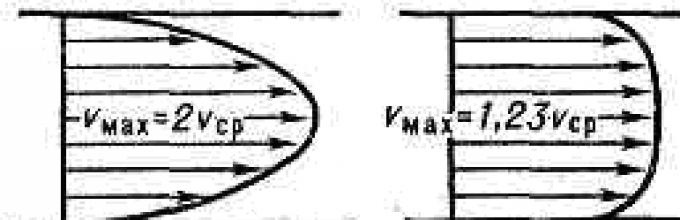
averaged velocity over the flow cross-section (Fig. 2) and integral characteristics - dependence of the average over the cross-section or max. speed, flow rate, as well as coefficient. resistance from the Reynolds number Re, the profile of the average speed of thermal energy in pipes or channels differs from parabolic. profile of the corresponding laminar flow with a faster increase in velocity at the walls and lower

Rice. 2. Average velocity profile: a - for laminar flow; b - in turbulent flow.

curvature to the center. parts of the flow. With the exception of a thin layer near the wall, the velocity profile is described logarithmically. law (i.e. linearly depends on the logarithm of the distance to the wall). Coeff. resistance l=8tw/rv2cp (where tw is the friction on the wall, r is the fluid, vav is the cross-sectional average flow velocity) is related to Re by the relation:

l1/2 = (1/c?8) ln (l1/2Re)+B,

where c. and B are numerical constants. Unlike laminar boundary layers, turbulent ones usually have a distinct boundary that fluctuates randomly with time (within 0.4 b - 1.2 d, where d is the distance from the wall, at which the average speed is 0.99 v, and v - speed outside the boundary layer). The average velocity profile in the near-wall part of the turbulent boundary layer is described logarithmically. law, and in external part, the speed increases with distance from the wall faster than logarithmically. law. The dependence of l on Re here has a form similar to that indicated above.

Jets, wakes and mixing zones have approx. self-similarity: in each section c = const of any of these T. t. at not too small distances x from the beginning. sections, one can introduce such scales of length and velocity L(x) and v(x) that the dimensionless statistical hydrodynamic characteristics fields (in particular, average velocity profiles) obtained by applying these scales will be the same in all sections.

In the case of free flow currents, the area of flow occupied by vortex flow flows at each moment of time has a clear, but very irregularly shaped boundary, outside of which flow is potential. The zone of intermittent turbulence turns out to be much wider here than in the boundary layers.

Physical encyclopedic dictionary. - M.: Soviet Encyclopedia. . 1983 .

TURBULENT FLOW

The form of flow of a liquid or gas, with a cut due to the presence of numerous flows. vortices decomposition sizes, liquid particles perform chaotic behavior. unsteady movements along complex trajectories (see. Turbulence), in contrast to laminar flows with smooth quasi-parallel particle trajectories. T. t. are observed at certain. conditions (at sufficiently large Reynolds numbers) in pipes, channels, boundary layers near the surfaces of solid bodies moving relative to a liquid or gas, in the wake of such bodies, jets, mixing zones between flows of different speeds, as well as in a variety of natural conditions.

T. T. differ from laminar not only in the nature of the movement of particles, but also in the distribution of the average velocity over the cross section of the flow, the dependence of the average or max. speed, flow and coefficient resistance from Reynolds number Re, much greater intensity of heat and mass transfer.

The profile of the average speed of thermal energy in pipes and channels differs from parabolic. profile of laminar flows with less curvature at the axis and a more rapid increase in velocity at the walls, where, with the exception of a thin viscous sublayer (thickness of the order of , where v- viscosity, - "friction speed", t-turbulent friction stress, r-density) the velocity profile is described by a universal Re logarithmic by law:

Where y 0 is equal for a smooth wall and proportional to the height of the tubercles for a rough wall.

A turbulent boundary layer, unlike a laminar boundary layer, usually has a distinct boundary that fluctuates irregularly in time within the limits where d is the distance from the wall, at which the speed reaches 99% of the value outside the boundary layer; in this region, the speed increases with distance from the wall faster than in logarithmic. law.

Jets, wakes and mixing zones have approx. self-similarity: with distance x from the beginning section length scale L grows like x t, and the speed scale U decreases as x-n, where for a volumetric jet t = n = 1, for flat T=1, n=1/2, for volumetric trace T= 1/3, n= 2/3, for a flat trace t=n=1/2, for mixing zone m= 1, n = 0. The boundary of the turbulent region here is also distinct, but irregular in shape and fluctuates wider than that of the boundary layers, in a flat wake - in the range (0.4-3.2) L.

Lit.: Landau L.D., Lifshits E.M., Mechanics of Continuous Media, 2nd ed., M., 1954; Loytsyansky L.G., Mechanics of liquid and gas, 6th ed., M., 1987; Townsend A. A., Structure of turbulent flow with transverse shear, trans. from English, M., 1959; Abramovich G.N., Theory of turbulent jets, M., 1960; Monin A. S., Yaglom A. M., Statistical, 2nd ed., h . 1, St. Petersburg, 1992. A. S. Monin.

Physical encyclopedia. In 5 volumes. - M.: Soviet Encyclopedia. Editor-in-chief A. M. Prokhorov. 1988 .

See what “TURBULENT FLOW” is in other dictionaries:

The flow of a liquid or gas, characterized by chaotic, irregular movement of its volumes and their intense mixing (see Turbulence), but generally having a smooth, regular character. The formation of T. t. is associated with instability... ... Encyclopedia of technology

- (from the Latin turbulentus, stormy, disorderly), the flow of a liquid or gas, in which the particles of the liquid make disordered, chaotic movements along complex trajectories, and the speed, temperature, pressure and density of the medium experience chaotic... ... Big Encyclopedic Dictionary

Modern encyclopedia

TURBULENT FLOW, in physics, the movement of a fluid medium in which random movement of its particles occurs. Characteristic of a liquid or gas with a high REYNOLDS NUMBER. see also LAMINAR FLOW... Scientific and technical encyclopedic dictionary

turbulent flow- A flow in which gas particles move in a complex, disordered manner and transport processes occur at the macroscopic rather than at the molecular level. [GOST 23281 78] Topics: aerodynamics of aircraft Generalizing terms, types of flows... ... Technical Translator's Guide

Turbulent flow- (from the Latin turbulentus stormy, disorderly), the flow of a liquid or gas, in which the particles of the liquid make disordered, chaotic movements along complex trajectories, and the speed, temperature, pressure and density of the medium are experienced... ... Illustrated Encyclopedic Dictionary

- (from Latin turbulentus stormy, disorderly * a. turbulent flow; n. Wirbelstromung; f. ecoulement turbulent, ecoulement tourbillonnaire; i. flujo turbulento, corriente turbulenta) the movement of a liquid or gas, during which and ... ... Geological encyclopedia

turbulent flow- A form of flow of water or air in which its particles make disordered movements along complex trajectories, which leads to intense mixing. Syn.: turbulence… Dictionary of Geography

TURBULENT FLOW- a type of liquid (or gas) flow in which their small volumetric elements perform unsteady movements along complex random trajectories, which leads to intense mixing of layers of liquid (or gas). T. t. arises as a result... ... Big Polytechnic Encyclopedia

Continuum mechanics Continuum Classical mechanics Law of conservation of mass Law of conservation of momentum ... Wikipedia

Studying the properties of liquid and gas flows is very important for industry and utilities. Laminar and turbulent flow affects the speed of transportation of water, oil, and natural gas through pipelines for various purposes and affects other parameters. The science of hydrodynamics deals with these problems.

Classification

In the scientific community, the flow regimes of liquids and gases are divided into two completely different classes:

laminar (jet);
turbulent.

A transition stage is also distinguished. By the way, the term “liquid” has a broad meaning: it can be incompressible (this is actually a liquid), compressible (gas), conducting, etc.

Background

Even Mendeleev in 1880 expressed the idea of the existence of two opposite flow regimes. This issue was studied in more detail by the British physicist and engineer Osborne Reynolds, completing his research in 1883. First practically, and then using formulas, he established that at low flow speeds, the movement of liquids takes on a laminar form: layers (particle flows) hardly mix and move along parallel trajectories. However, after overcoming a certain critical value (it is different for different conditions), called the Reynolds number, the fluid flow regimes change: the jet flow becomes chaotic, vortex - that is, turbulent. As it turned out, these parameters are also characteristic of gases to a certain extent.

Practical calculations of the English scientist showed that the behavior of, for example, water strongly depends on the shape and size of the reservoir (pipe, channel, capillary, etc.) through which it flows. Pipes with a circular cross-section (such as are used for the installation of pressure pipelines) have their own Reynolds number - the formula is described as follows: Re = 2300. For flow along an open channel, it is different: Re = 900. At lower values of Re, the flow will be ordered, at higher values - chaotic .

Laminar flow

The difference between laminar flow and turbulent flow is the nature and direction of water (gas) flows. They move in layers, without mixing and without pulsations. In other words, the movement occurs evenly, without random jumps in pressure, direction and speed.

Laminar flow of liquid is formed, for example, in narrow living beings, capillaries of plants and, under comparable conditions, during the flow of very viscous liquids (fuel oil through a pipeline). To clearly see the jet flow, just open the water tap slightly - the water will flow calmly, evenly, without mixing. If the tap is turned off all the way, the pressure in the system will increase and the flow will become chaotic.

Turbulent flow

Unlike laminar flow, in which nearby particles move along almost parallel trajectories, turbulent fluid flow is disordered. If we use the Lagrange approach, then the trajectories of particles can intersect arbitrarily and behave quite unpredictably. The movements of liquids and gases under these conditions are always nonstationary, and the parameters of these nonstationarities can have a very wide range.

How the laminar regime of gas flow turns into turbulent can be traced using the example of a stream of smoke from a burning cigarette in still air. Initially, the particles move almost parallel along trajectories that do not change over time. The smoke seems motionless. Then, in some place, large vortices suddenly appear and move completely chaotically. These vortices break up into smaller ones, those into even smaller ones, and so on. Eventually, the smoke practically mixes with the surrounding air.

Turbulence cycles

The example described above is textbook, and from its observation, scientists have drawn the following conclusions:

Laminar and turbulent flow are probabilistic in nature: the transition from one regime to another does not occur in a precisely specified place, but in a rather arbitrary, random place.
First, large vortices appear, the size of which is larger than the size of a stream of smoke. The movement becomes unsteady and highly anisotropic. Large flows lose stability and break up into smaller and smaller ones. Thus, a whole hierarchy of vortices arises. The energy of their movement is transferred from large to small, and at the end of this process disappears - energy dissipation occurs at small scales.
The turbulent flow regime is random in nature: one or another vortex can end up in a completely arbitrary, unpredictable place.
Mixing of smoke with the surrounding air practically does not occur in laminar conditions, but in turbulent conditions it is very intense.
Despite the fact that the boundary conditions are stationary, the turbulence itself has a pronounced non-stationary character - all gas-dynamic parameters change over time.

There is another important property of turbulence: it is always three-dimensional. Even if we consider a one-dimensional flow in a pipe or a two-dimensional boundary layer, the movement of turbulent vortices still occurs in the directions of all three coordinate axes.

Reynolds number: formula

The transition from laminarity to turbulence is characterized by the so-called critical Reynolds number:

Re cr = (ρuL/µ) cr,

where ρ is the flow density, u is the characteristic flow speed; L is the characteristic size of the flow, µ is the coefficient cr - flow through a pipe with a circular cross-section.

For example, for a flow with speed u in a pipe, L is used as Osborne Reynolds showed that in this case 2300

A similar result is obtained in the boundary layer on the plate. The distance from the leading edge of the plate is taken as a characteristic size, and then: 3 × 10 5

Concept of speed disturbance

Laminar and turbulent fluid flow, and, accordingly, the critical value of the Reynolds number (Re) depend on a large number of factors: pressure gradient, height of roughness tubercles, intensity of turbulence in the external flow, temperature difference, etc. For convenience, these total factors are also called velocity disturbance , since they have a certain effect on the flow rate. If this disturbance is small, it can be extinguished by viscous forces tending to level the velocity field. With large disturbances, the flow may lose stability and turbulence occurs.

Considering that the physical meaning of the Reynolds number is the ratio of inertial forces and viscous forces, the disturbance of flows falls under the formula:

Re = ρuL/µ = ρu 2 /(µ×(u/L)).

The numerator contains double the velocity pressure, and the denominator contains a quantity of the order of friction stress if the thickness of the boundary layer is taken as L. The high-speed pressure tends to destroy the balance, but this is counteracted. However, it is not clear why (or the velocity pressure) leads to changes only when they are 1000 times greater than the viscous forces.

Calculations and facts

It would probably be more convenient to use the velocity disturbance rather than the absolute flow velocity u as the characteristic velocity in Recr. In this case, the critical Reynolds number will be of the order of 10, that is, when the disturbance of the velocity pressure exceeds the viscous stresses by 5 times, the laminar flow of the fluid becomes turbulent. This definition of Re, according to a number of scientists, well explains the following experimentally confirmed facts.

For an ideally uniform velocity profile on an ideally smooth surface, the traditionally determined number Re cr tends to infinity, that is, the transition to turbulence is actually not observed. But the Reynolds number, determined by the magnitude of the speed disturbance, is less than the critical one, which is equal to 10.

In the presence of artificial turbulators that cause a burst of speed comparable to the main speed, the flow becomes turbulent at much lower values of the Reynolds number than Re cr determined from the absolute value of the speed. This makes it possible to use the value of the coefficient Re cr = 10, where the absolute value of the speed disturbance caused by the above reasons is used as the characteristic speed.

Stability of laminar flow in a pipeline

Laminar and turbulent flow is characteristic of all types of liquids and gases under different conditions. In nature, laminar flows are rare and are characteristic, for example, of narrow underground flows in flat conditions. This issue worries scientists much more in the context of practical applications for transporting water, oil, gas and other technical liquids through pipelines.

The issue of laminar flow stability is closely related to the study of the perturbed motion of the main flow. It has been established that it is exposed to so-called small disturbances. Depending on whether they fade or grow over time, the main flow is considered stable or unstable.

Flow of compressible and incompressible fluids

One of the factors influencing laminar and turbulent flow of a fluid is its compressibility. This property of a liquid is especially important when studying the stability of unsteady processes with a rapid change in the main flow.

Research shows that laminar flow of incompressible fluid in pipes of cylindrical cross-section is resistant to relatively small axisymmetric and non-axisymmetric disturbances in time and space.

Recently, calculations have been carried out on the influence of axisymmetric disturbances on the stability of the flow in the inlet part of a cylindrical pipe, where the main flow depends on two coordinates. In this case, the coordinate along the pipe axis is considered as a parameter on which the velocity profile along the pipe radius of the main flow depends.

Conclusion

Despite centuries of study, it cannot be said that both laminar and turbulent flow have been thoroughly studied. Experimental studies at the micro level raise new questions that require reasoned computational justification. The nature of the research also has practical benefits: thousands of kilometers of water, oil, gas, and product pipelines have been laid throughout the world. The more technical solutions are implemented to reduce turbulence during transportation, the more effective it will be.

TURBULENT FLOW TURBULENT FLOW (from the Latin turbulentus - stormy, chaotic), the flow of a liquid or gas in which the particles of the liquid make disordered, chaotic movements along complex trajectories, and the speed, temperature, pressure and density of the medium experience chaotic fluctuations. It differs from laminar flow in intense mixing, heat exchange, high values of the friction coefficient, etc. In nature and technology, most flows of liquids and gases are turbulent flows.

Modern encyclopedia. 2000 .

See what “TURBULENT FLOW” is in other dictionaries:

- (from Latin turbulentus stormy, disorderly), the form of flow of a liquid or gas, when its elements perform unsteady movements along complex trajectories, which leads to intense mixing between layers of liquid or gas (see... ... Physical encyclopedia

Continuum mechanics Continuum Classical mechanics Law of conservation of mass Law of conservation of momentum ... Wikipedia

At sufficiently large Reynolds numbers, the fluid motion ceases to be laminar; Thus, in pipes with smooth walls, laminar movement becomes turbulent at numbers

In this movement, the hydrodynamic parameters begin to fluctuate around their average values, mixing of the liquid occurs and its flow becomes random. The movement of air in the atmosphere and water in the ocean, when the Reynolds numbers are high (and they can reach in certain conditions), is almost always turbulent. In technical problems of aero- and hydromechanics it is extremely common to encounter such motion; The numbers here can reach values as well. For this reason, great attention has always been paid to the study of turbulence. However, although turbulent motion, starting with the work of Reynolds, has been studied for about a century and by now we already know a lot about the features and patterns of this motion, we cannot yet say that there is a complete understanding of this complex physical phenomenon.

The question of the emergence and development of turbulent motion has not yet been sufficiently clarified, although there is no doubt that it is associated with the instability of the flow at large numbers due to the nonlinearity of the hydrodynamic equations; We will briefly discuss this below. For us, however, when studying the propagation of waves in a turbulent medium, information about an already developed, steady turbulent flow, its internal structure and dynamic patterns will be of greater importance.

Great success in modern ideas about already developed turbulent flow was achieved in 1941 by A. N. Kolmogorov and A. M. Obukhov, who were credited with creating a general diagram of the mechanism of such a turbulent flow at high Reynolds numbers, elucidating its internal structure and a number of statistical patterns. Since then, the development of the statistical theory of turbulence and related experiments has led to a number of significant results. A detailed presentation of the modern statistical theory of turbulence and its experimental research is given in the works. This theory turned out to be important for the problem of "turbulence and waves" both for the propagation of acoustic waves in the atmosphere and sea, and for the propagation of electromagnetic waves in the atmosphere, ionosphere and plasma. Here we will limit ourselves to a brief presentation of only the most basic information about this theory, which we will need in the future.

In 1920, the English hydromechanic and meteorologist L. F. Richardson expressed a fruitful hypothesis, which is called the hypothesis of “grinding” turbulence. He suggested that in the case of atmospheric turbulence, when large masses of air move, for some reason, for example due to surface roughness, the flow becomes unstable and large velocity pulsations or vortices are formed. These vortices draw their energy from the energy of the entire flow as a whole. The characteristic sizes of these vortices

L is the same scale as the scale of the flow itself (the external scale of turbulence). But at sufficiently large scales of motion and flow velocities, these vortices themselves become unstable and break up into smaller vortices on the scale of the Reynolds number for such vortices where the pulsations of their speed are large and they, in turn, break up into smaller ones. This process of “grinding” turbulent inhomogeneities continues further and further: the energy of large vortices, coming from the energy of the flow, is transferred to ever smaller vortices, down to the smallest ones, having an internal scale of I, when the viscosity of the liquid begins to play a significant role (numbers for such vortices small, their movement is stable). The energy of the smallest possible vortices is converted into heat.

This Richardson hypothesis was developed in the works of A. N. Kolmogorov and his school.

In the inertial region of pulsation scales, we can assume that viscosity does not play a role, energy simply flows from large scales to smaller ones, and the dissipation of energy per unit volume of liquid per unit time is some function of only changes in the average speed over distances of the order of I, the scale I itself and density, t .e.

Of the three quantities, only one combination can be made, having the dimension :

From this relationship we can estimate the order of change in the average speed of turbulent motion over a distance of order I:

Since in the considered inertial spectral interval of vortices, starting from the outer scale L and ending with the inner scale 1 (where viscosity plays a decisive role), the value is constant, then

where C is a constant, which for conditions of atmospheric turbulence and turbulence in a wind tunnel (behind the grid) is of the order of magnitude and increases with increasing flow speed u. The root mean square of the velocity difference at points 1 and 2 (or the so-called structure function) in a turbulent flow will thus be

where is the distance between observation points 1 and 2. This is the so-called Kolmogorov-Obukhov law of two-thirds (A. M. Obukhov came to the formulation of such a law from spectral concepts).

It should be noted that L. Onsager, K. Weizsäcker and W. Heisenberg also later came to the same law.

In the above arguments, based on considerations of similarity and dimensions, it is assumed that the flow as a whole does not have an orienting effect on the vortices: therefore, the movement of vortices in the inertial subregion of the pulsation spectrum can be approximately considered locally homogeneous and isotropic, which will also be discussed in Chapter. 7. For this reason, the statistical theory of turbulence is called the theory of locally isotropic turbulence.

The “two-thirds” law applies to the turbulent pulsation field, i.e., to the vector random field, and, generally speaking, it is necessary to clarify which components of v in (7.5) we are dealing with.

Temperature pulsations, which are also present in a dynamic turbulent flow (temperature inhomogeneities), are mixed by pulsations of the velocity field. For the scalar temperature field of pulsations, the mechanism of refinement of inhomogeneities by pulsations of the velocity field also operates; the size of the smallest temperature inhomogeneities is limited by the action of thermal conductivity, just as in the field of velocity pulsations the minimum scale of vortices is determined by viscosity.

For the temperature field of pulsations in a dynamic flow, A. M. Obukhov obtained the “two-thirds” law, which has a form similar to (7.5):

where is a constant depending on speed .

In the interval of internal scales I (this interval is called the equilibrium interval), the value will be a function not only of , but also of kinematic viscosity

Then the only combination that has dimension will be the following expression for:

(7.8)

Respectively

where , i.e. in this case there is a quadratic dependence on (Taylor's law).

The internal turbulence scale I itself can be estimated from relation (7.4), assuming that (7.4) is valid up to the conditions

A complete picture of the behavior of the structure function of the velocity field depending on the distance between observation points is shown

in Fig. 1.5. At small scales of velocity pulsations corresponding to the internal scale, the structure function obeys Taylor's quadratic law (equilibrium interval). When increasing, the function obeys the law of “two thirds” (inertial interval; it is also called the inertial subregion of the pulsation spectrum); with a further increase, when the initial provisions cease to be valid.

Rice. 1.5. Structural function of the velocity field.

Note that the law of “two thirds” takes place not only for pulsations of the velocity field and the field of temperature pulsations (considered as a passive admixture), but also for pulsations of humidity, also considered as a passive admixture

for pressure pulsations

These are some of the conclusions that are significant for us, which were obtained on the basis of Richardson's hypothesis and considerations of the theory of similarity and dimension or from spectral concepts.

In the “two-thirds” law, you should pay attention to the fact that it takes the root mean square of the difference in velocities at two points in the flow, or the so-called “structure function” of the velocity field. There is a deep meaning in this.

If you measure (record) velocity or temperature pulsations at one point in the flow, then large inhomogeneities will play a larger role than small ones, and the measurement results will significantly depend on the time during which these measurements are made. This difficulty disappears if you measure the difference in speeds at two relatively close points of the flow, i.e., monitor the relative motion of two close elements of the flow. This difference will not be affected by large eddies whose size is much larger than the distance between these two points.

Unlike the kinetic theory of gases, when it can be assumed as a first approximation that the movement of each molecule does not depend on the molecules located in its immediate vicinity, in a turbulent flow the situation is different. Adjacent fluid elements tend to assume the same velocity value as the element in question unless the distance between them is small. If we consider a turbulent flow as a superposition of pulsations

(vortices) of different scales, then the distance between two, close elements will first change due to only the smallest vortices. Large vortices will simply transport the pair of points (elements) in question as a whole, without trying to separate them. But as soon as the distance between the fluid elements increases, in addition to the small ones, larger vortices come into play. Therefore, in a turbulent fluid flow, it is not so much the movement of the fluid element itself that is important, but rather the change in its distance from neighboring elements.

After we have become acquainted with the basic concepts of the internal structure of a developed turbulent flow, let us return to the issue of the emergence of turbulence, i.e., the transition from laminar to turbulent motion (in modern literature, the abbreviated term “transition” is used for this phenomenon).

The nonlinear process of energy exchange between different degrees of freedom, essentially inherent in Richardson’s model of the cascade process of energy conversion and improved by A. N. Kolmogorov, led L. D. Landau to a model in which this transition was associated with the excitation in a hydrodynamic system of an ever-increasing number of degrees freedom. There are certain difficulties in this interpretation of the transition. A step forward in overcoming them was made by A. M. Obukhov and his colleagues 121, 22] and A. S. Monin on the basis of a theoretical and experimental study of the simplest system that has the general properties of hydrodynamic equations (quadratic nonlinearity and conservation laws). Such a system is a system with three degrees of freedom (triplet), the equations of motion of which coincide in the corresponding coordinate system with the Euler equations in the theory of the gyroscope. The hydrodynamic interpretation of the triplet can be “fluid rotation” in an incompressible fluid inside a triaxial ellipsoid, in which the velocity field is linear in coordinates.

The elementary mechanism of nonlinear energy conversion between different degrees of freedom in such a triplet, which has been verified experimentally, can be used as the basis for modeling more complex systems (cascade of triplets) to explain the cascade process of energy conversion according to the Richardson-Kolmogorov-Landau scheme. One can hope that some progress will be achieved along this path in the near future.

Another way to explain the transition, which has been developed recently, is related to the fact that stochasticity is possible not only in extremely complex dynamic systems in which absolutely accurate initial conditions cannot really be specified, and therefore there is a need for a statistical description. It became clear that these established ideas about the nature of chaos are not always correct. Chaotic behavior has also been found in much simpler systems, including systems described by just three first-order ordinary differential equations. Despite the fact that this discovery is immediately

stimulated a number of studies in the field of mathematical theory of the complex behavior of simple dynamic systems; only in the mid-seventies did it attract the attention of a wide range of physicists, mechanics, and biologists. Around the same time, chaos in simple systems was compared with the problem of the emergence of turbulence. Further, stochastic self-oscillations were discovered in a wide variety of, sometimes very unexpected, areas, and their mathematical image - a strange attractor - has now taken a prominent place in the qualitative theory of dynamical systems along with the well-known attractors - equilibrium states and limit cycles. To what extent this direction will contribute to the development of transition theory is not yet entirely clear.

TURBULENT is a flow accompanied by intense mixing of a liquid with pulsations of speeds and pressures. Along with the main longitudinal movement of the liquid, transverse movements and rotational movements of individual volumes of liquid are observed.

Turbulent fluid flow observed under certain conditions (at sufficiently large numbers Reynolds) in pipes, channels, boundary layers near the surfaces of solid bodies moving relative to a liquid or gas, in the wake of such bodies, jets, mixing zones between flows of different speeds, as well as in a variety of natural conditions.

T.t. differ from laminar not only in the nature of the movement of particles, but also in the distribution of the average velocity over the flow cross section, the dependence of the average or max. speed, flow and coefficient resistance from Reynolds number Re, much greater intensity of heat and mass transfer. Average speed profile T.t. in pipes and channels differs from parabolic. profile of laminar flows with less curvature at the axis and a more rapid increase in velocity at the walls.

Pressure loss during turbulent fluid movement

All hydraulic energy losses are divided into two types: friction losses along the length of pipelines and local losses caused by such pipeline elements in which, due to changes in the size or configuration of the channel, the flow velocity changes, the flow is separated from the walls of the channel and vortex formation occurs.

The simplest local hydraulic resistance can be divided into expansions, contractions and turns of the channel, each of which can be sudden or gradual. More complex cases of local resistance are compounds or combinations of the simplest resistances listed.

In a turbulent regime of fluid movement in pipes, the velocity distribution diagram has the form shown in Fig. In a thin near-wall layer of thickness δ, the liquid flows in laminar mode, and the remaining layers flow in turbulent mode, and are called turbulent core. Thus, strictly speaking, turbulent motion does not exist in its pure form. It is accompanied by laminar motion near the walls, although the laminar layer δ is very small compared to the turbulent core.

Model of turbulent fluid motion

The main calculation formula for pressure losses during turbulent fluid flow in round pipes is the empirical formula already given above, called the Weisbach-Darcy formula and having the following form:

The difference lies only in the values of the hydraulic friction coefficient λ. This coefficient depends on the Reynolds number Re and on the dimensionless geometric factor - the relative roughness Δ/d (or Δ/r 0, where r 0 is the radius of the pipe).

Critical Reynolds number

The Reynolds number at which a transition from one mode of fluid motion to another occurs is called critical. At Reynolds number a laminar mode of motion is observed, at the Reynolds number - turbulent regime of fluid movement. More often, the critical value of a number is taken to be , this value corresponds to the transition of fluid motion from turbulent to laminar. When transitioning from laminar to turbulent fluid flow, the critical value is greater. The critical value of the Reynolds number increases in pipes that narrow and decreases in those that expand. This is because as the cross-section becomes narrower, the velocity of the particles increases, so the tendency for transverse movement decreases.

Thus, the Reynolds similarity criterion allows us to judge the fluid flow regime in the pipe. At Re< Re кр течение является ламинарным, а при Re >Re flow is turbulent. More precisely, a fully developed turbulent flow in pipes is established only when Re is approximately equal to 4000, and at Re = 2300...4000 there is a transitional, critical region.

As experience shows, for round pipes Re cr is approximately equal to 2300.

The mode of fluid movement directly affects the degree of hydraulic resistance of pipelines.

For laminar mode

For turbulent mode