By definition, the differential (first differential) of a function is calculated by the formula  If
If  is an independent variable.
EXAMPLE.
Let us show that the form of the first differential remains unchanged (it is invariant) even in the case when the function argument  itself is a function, that is, for complex function
 .
.
Let  are differentiable, then by definition
In addition, as required to prove.
EXAMPLES.

The proven invariance of the form of the first differential allows us to assume that  that is the derivative is equal to the ratio of the differential of the function to the differential of its argument, regardless of whether the argument is an independent variable or a function.
Differentiation of a function defined parametrically
Let If function  has on set
  reverse, then
  Then the equalities
  defined on the set
  a function defined parametrically,
  –
parameter (intermediate variable).
–
parameter (intermediate variable).
EXAMPLE. Plot a function  .
.

|
About 1 |
 y
y
 x
xThe constructed curve is called cycloid(Fig. 25) and is the trajectory of a point on a circle of radius 1 that rolls without slip along the OX axis.
COMMENT. Sometimes, but not always, a parameter can be eliminated from the parametric curve equations.
EXAMPLES.
 – parametric equations circles, since, obviously,
 are the parametric equations of the ellipse, since
 are the parametric equations of the parabola
Find the derivative of a function given parametrically:

The derivative of a function defined parametrically is also a function defined parametrically:  .
.
DEFINITION. The second derivative of a function is called the derivative of its first derivative.
derivative  -th order is the derivative of its order derivative
  .
.
denote the derivatives of the second and  th order like this:
It follows from the definition of the second derivative and the rule of differentiation of a parametrically given function that  To calculate the third derivative, it is necessary to represent the second derivative in the form
  and use the resulting rule again. Higher order derivatives are calculated in a similar way.
EXAMPLE. Find first and second order derivatives of a function
 .
.
Basic theorems of differential calculus
THEOREM(Farm). Let the function  has at the point
  extremum. If exists
  , That
PROOF. Let  , for example, is the minimum point. By definition of a minimum point, there is a neighborhood of this point
  , within which
  , that is
  - increment
  at the point
  . A-priory
  Calculate one-sided derivatives at a point
  :
:
 by the passage to the limit theorem in the inequality,
because 
 , because
  But by condition
  exists, so the left derivative is equal to the right one, and this is possible only if
The assumption that  - the maximum point, leads to the same.
The geometric meaning of the theorem:
THEOREM(Roll). Let the function  continuous
  , differentiable
  And
And  then there is
  such that
PROOF. Because  continuous
  , then by the second Weierstrass theorem it reaches
  their greatest
  and least
  values either at the extremum points or at the ends of the segment.
1. Let  , Then
2. Let  Because
  either
  , or
, or  reached at the extreme point
  , but by Fermat's theorem
  Q.E.D.
THEOREM(Lagrange). Let the function  continuous
  and differentiable
  , then there exists
  such that
  .
.
The geometric meaning of the theorem:
Because  , then the secant is parallel to the tangent. Thus, the theorem states that there is a tangent parallel to a secant passing through points A and B.
PROOF. Through points A  and B
and B  draw a secant AB. Her Equation
  Consider the function
 - the distance between the corresponding points on the graph and on the secant AB.
1.
 continuous
  as the difference of continuous functions.
2.
 differentiable
  as the difference of differentiable functions.
3.

Means,  satisfies the conditions of Rolle's theorem, so there exists
  such that
The theorem has been proven.
COMMENT. The formula is called Lagrange formula.
THEOREM(Koshi). Let the functions  continuous
  , differentiable
  And
And  , then there is a point
  such that
  .
.
PROOF. Let us show that  . If
. If  , then the function
  would satisfy the condition of Rolle's theorem, so there would be a point
  such that
  is a contradiction to the condition. Means,
  , and both parts of the formula are defined. Let's consider an auxiliary function.
 continuous
  , differentiable
  And
And  , that is
  satisfies the conditions of Rolle's theorem. Then there is a point
  , wherein
  , But
, But
Q.E.D.
The proven formula is called Cauchy formula.
L'Hopital's RULE(Theorem L'Hopital-Bernoulli). Let the functions  continuous
  , differentiable
  ,
, And
And  . In addition, there is a finite or infinite
  .
.
Then there is 
PROOF. Since according to the condition  , then we define
  at the point
  , assuming
  Then
Then  become continuous
  . Let us show that
 Let's pretend that
  then there is
  such that
  , since the function
  on
on  satisfies the conditions of Rolle's theorem. But by condition
  - a contradiction. That's why
 . Functions
  satisfy the conditions of the Cauchy theorem on any interval
  , which is contained in
  . Let's write the Cauchy formula:
 ,
,
 .
.
Hence we have:  , because if
  , That
  .
.
Renaming the variable in the last limit, we obtain the required:

NOTE 1. L'Hopital's rule remains valid even when  And
And  . It allows you to reveal not only the uncertainty of the form
  , but also of the form
  :
:
 .
.
NOTE 2. If, after applying the L'Hopital rule, the uncertainty is not revealed, then it should be applied again.
EXAMPLE.
COMMENT 3 . L'Hopital's rule is a universal way to reveal uncertainties, but there are limits that can be revealed by applying only one of the previously studied particular techniques.
But obviously  , since the degree of the numerator is equal to the degree of the denominator, and the limit is equal to the ratio coefficients at higher powers
Function differential
The function is called differentiable at a point, limiting for the set E, if its increment Δ f(x 0) corresponding to the increment of the argument x, can be represented as
Δ f(x 0) = A(x 0)(x - x 0) + ω (x - x 0), (1)
Where ω (x - x 0) = O(x - x 0) at x → x 0 .
Display, called differential functions f at the point x 0 , and the value A(x 0)h - differential value at this point.
For the value of the function differential f accepted designation df or df(x 0) if you want to know at what point it was calculated. Thus,
df(x 0) = A(x 0)h.
Dividing in (1) by x - x 0 and aiming x To x 0 , we get A(x 0) = f"(x 0). Therefore we have
df(x 0) = f"(x 0)h. (2)
Comparing (1) and (2), we see that the value of the differential df(x 0) (when f"(x 0) ≠ 0) yes main part function increments f at the point x 0 , linear and homogeneous at the same time with respect to increment h = x - x 0 .
Function differentiability criterion
In order for the function f was differentiable at a given point x 0 , it is necessary and sufficient that it has a finite derivative at this point.
Invariance of the form of the first differential
If x is an independent variable, then dx = x - x 0 (fixed increment). In this case we have
df(x 0) = f"(x 0)dx. (3)
If x = φ (t) is a differentiable function, then dx = φ" (t 0)dt. Hence,
We have seen that the differential of a function can be written as:
 (1),
(1),
If  is an independent variable. Let now
  there is a complex function
  , i.e.
  ,
, and therefore
  . If the derivatives of the functions
  And
And  exist, then
  , as a derivative of a complex function. Differential
  or. But
  and therefore we can write
  , i.e. get the expression for
  as in (1).
Conclusion: formula (1) is correct as in the case when  is an independent variable, and in the case when
  is a function of the independent variable
  . In the first case under
  is understood as the differential of the independent variable
  , in the second - the differential of the function (in this case
  , generally speaking). This shape-preserving property (1) is called differential form invariance.
The invariance of the form of the differential gives great benefits when calculating the differentials of complex functions.
For example: to be calculated  . Whether dependent or independent variable
  , we can write. If
  - function, for example
  , then we find
  and, using the invariance of the form of the differential, we have the right to write down.
§18. Derivatives of higher orders.
Let the function y \u003d (x) be differentiable on some interval X, (i.e., it has a finite derivative y 1 \u003d 1 (x) at each point of this interval). Then 1 (x) is in X itself a function of x. It may turn out that at some points or at all x 1 (x) itself has a derivative, i.e. there is a derivative of the derivative (y 1) 1 \u003d ( 1 (x) 1. In this case, it is called the second derivative or second-order derivative. They are denoted by the symbols y 11, 11 (x), d 2 y / dx 2. If necessary emphasize that the derivative is in m.x 0, then write
y 11 / x \u003d x 0 or 11 (x 0) or d 2 y / dx 2 / x \u003d x 0
the derivative of y 1 is called the first order derivative or the first derivative.
So, the second-order derivative is the derivative of the first-order derivative of a function.
Quite similarly, the derivative (where it exists) of the second order derivative is called the third order derivative or the third derivative.
Designate (y 11) 1 \u003d y 111 \u003d 111 (x) \u003d d 3 y / dx 3 \u003d d 3 (x) / dx 3
In general, the derivative of the n-th order of the function y \u003d (x) is the derivative of the derivative (n-1) of the order of this function. (if they exist, of course).
designate
Read: n-th derivative of y, from (x); d n y by d x in the n-th.
Fourth, fifth, etc. it is inconvenient to indicate the order with strokes, therefore they write the number in brackets, instead of v (x) they write (5) (x).
In brackets, so as not to confuse the nth order of the derivative and the nth degree of the function.
Derivatives of order higher than the first are called derivatives of higher orders.
It follows from the definition itself that to find the nth derivative, you need to find successively all the previous ones from the 1st to the (n-1)th.
Examples: 1) y \u003d x 5; y 1 \u003d 5x 4; y 11 \u003d 20x 3;
y 111 \u003d 60x 2; y (4) =120x; y (5) =120; y (6) =0,…
2) y=e x; y 1 \u003d e x; y 11 \u003d e x; ...;
3) y=sinx; y 1 = cosx; y 11 = -sinx; y 111 = -cosx; y (4) = sinх;…
Note that the second derivative has a certain mechanical meaning.
If the first derivative of the path with respect to time is the speed of non-uniform rectilinear motion
V=ds/dt, where S=f(t) is the equation of motion, then V 1 =dV/dt= d 2 S/dt 2 is the rate of change of speed, i.e. movement acceleration:
a \u003d f 11 (t) \u003d dV / dt \u003d d 2 S / dt 2.
So, the second derivative of the path with respect to time is the acceleration of the movement of the point - this is the mechanical meaning of the second derivative.
In a number of cases, it is possible to write an expression for a derivative of any order, bypassing intermediate ones.
Examples:
y=e x; (y) (n) = (e x) (n) = e x;
y=a x; y 1 \u003d a x lna; y 11 \u003d a x (lna) 2; y (n) = a x (lna) n;
y \u003d x α; y 1 \u003d αx α-1; y 11 =  ; y (p) \u003d α (α-1) ... (α-n + 1) x α-n, with
  =n we have
y (n) = (x n) (n) = n! The order derivatives above n are all zero.
y \u003d sinx; y 1 = cosx; y 11 = -sinx; y 111 = -cosx; y (4) = sinх;… etc.
y 1 \u003d sin (x +  /2); y 11 \u003d sin (x + 2
  /2); y 111 \u003d sin (x + 3
  /2); etc., then y (n) \u003d (sinx) (n) \u003d sin (x + n
  /2).
/2).
It is easy to establish by successive differentiation and general formulas:
1) (CU) (n) = C (U) (n) ; 2) (U ± V) (n) = U (n) ± V (n)
More complicated is the formula for the nth derivative of the product of two functions (U·V) (n) . It is called the Leibniz formula.
Let's get her
y \u003d U V; y 1 \u003d U 1 V + UV 1; y 11 \u003d U 11 V + U 1 V 1 + U 1 V 1 + UV 11 \u003d U 11 V + 2U 1 V 1 + UV 11;
y 111 \u003d U 111 V + U 11 V 1 + 2U 11 V 1 + 2U 1 V 11 + U 1 V 11 + UV 111 \u003d U 111 V + 3U 11 V 1 +3 U 1 V 11 + UV 111;
Similarly, we get
y (4) \u003d U (4) V + 4 U 111 V 1 +6 U 11 V 11 +4 U 1 V 111 + UV (4), etc.
It is easy to see that the right-hand sides of all these formulas resemble the expansion of the powers of the binomial U+V, (U+V) 2 , (U+V) 3 , etc. Only instead of the powers of U and V there are derivatives of the corresponding orders. The similarity will be especially complete if in the resulting formulas we write instead of U and V, U (0) and V (0) , i.e. 0th derivatives of the functions U and V (the functions themselves).
Extending this law to the case of any n, we obtain the general formula
y(n) = (UV)(n) = U(n) V+ n/1! U (n-1) V 1 + n(n-1)/2! U (n-2) V (2) + n(n-1)(n-2)/3! U (n-3) V (3) +…+ n(n-1)…(n-k+1)/K! U (k) V (n-k) + ... + UV (n) - Leibniz formula.
Example: find (e x x) (n)
(e x) (n) \u003d e x, x 1 \u003d 1, x 11 \u003d 0 and x (n) \u003d 0, therefore (e x x) (n) \u003d (e x) (n) x + n / 1 ! (e x) (n-1) x 1 \u003d e x x + ne x \u003d e x (x + n).