For this equation we have:
 ; (5.22)
 . (5.23)
The last determinant gives the condition a 3 > 0. The condition Δ 2 > 0, for a 0 > 0, a 1 > 0 and a 3 > 0, can only be satisfied for a 2 > 0.
Consequently, for a third-order equation, the positivity of all coefficients of the characteristic equation is no longer sufficient. It is also required to fulfill a certain relationship between the coefficients a 1 a 2 > a 0 a 3.
4. Fourth order equation
Similar to what was done above, we can obtain that for a fourth-order equation, in addition to the positivity of all coefficients, the following condition must be met:
A significant drawback of algebraic criteria, including the Hurwitz criteria, is also that for high-order equations, at best, one can get an answer as to whether the automatic control system is stable or unstable. Moreover, in the case of an unstable system, the criterion does not answer how the parameters of the system should be changed to make it stable. This circumstance led to the search for other criteria that would be more convenient in engineering practice.
5.3. Mikhailov stability criterion
Let us consider separately the left side of the characteristic equation (5.7), which is a characteristic polynomial
Let us substitute into this polynomial the purely imaginary value p = j, where represents the angular frequency of oscillations corresponding to the purely imaginary root of the characteristic solution. In this case we obtain the characteristic complex
where the real part will contain even powers of frequency
and imaginary – odd powers of frequency
E
Rice. 5.4. Mikhailov's hodograph
In practice, the Mikhailov curve is constructed point by point, and different values of frequency are specified and U() and V() are calculated using formulas (5.28), (5.29). The calculation results are summarized in table. 5.1.
Table 5.1
Construction of the Mikhailov curve
Using this table, the curve itself is constructed (Fig. 5.4).
Let us determine what the rotation angle of the vector D(j) should be equal to when the frequency changes from zero to infinity. To do this, we write the characteristic polynomial as a product of factors
where 1 – n are the roots of the characteristic equation.
The characteristic vector can then be represented as follows:
Each bracket represents a complex number. Therefore, D(j) is a product of n complex numbers. When multiplying, the arguments of complex numbers are added. Therefore, the resulting angle of rotation of the vector D(j) will be equal to the sum of the angles of rotation of the individual factors (5.31) as the frequency changes from zero to infinity
Let us define each term in (5.31) separately. To generalize the problem, consider different types of roots.
1. Let some root, for example 1, be real and negative , that is 1 = – 1 . The factor in expression (5.31), determined by this root, will have the form ( 1 + j). Let's construct a hodograph of this vector on the complex plane as the frequency changes from zero to infinity (Fig. 5.5, A). When= 0, the real part is U= 1, and the imaginary part is V= 0. This corresponds to point A, lying on the real axis. At0 the vector will change in such a way that its real part will still be equal to, and the imaginary part V = (point B on the graph). As the frequency increases to infinity, the vector goes to infinity, and the end of the vector always remains on the vertical straight line passing through point A, and the vector rotates counterclockwise.

Rice. 5.5. Real roots
The resulting angle of rotation of the vector 1 = +( / 2).
2. Let now the root 1 be real and positive , that is 1 = + 1.Then the factor in (5.31) determined by this root will have the form (– 1 + j). Similar constructions (Fig. 5.5, b) show that the resulting angle of rotation will be 1 = –( / 2). The minus sign indicates that the vector rotates clockwise.
3. Let two conjugate roots, for example 2 and 3, be complex with negative real part , that is 2;3 = –±j. Similarly, the factors in expression (5.31), determined by these roots, will have the form (–j + j)( + j + j).
At = 0, the initial positions of two vectors are determined by points A 1 and A 2 (Fig. 5.6, A). The first vector is rotated clockwise relative to the real axis by an angle equal to arctg( / ), and the second vector is rotated by the same angle counterclockwise. With a gradual increase in from zero to infinity, the ends of both vectors go up to infinity and both vectors ultimately merge with the imaginary axis.
The resulting angle of rotation of the first vector is 2 = ( / 2) + . The resulting angle of rotation of the second vector 3 = ( / 2) –. The vector corresponding to the product (–j + j)( + j + j) will rotate through the angle 2 + 3 = 2 / 2 =.

Rice. 5.6. Complex roots
4. Let them be the same complex roots have a positive real part , that is 2;3 = +±j.
Carrying out the construction similarly to the previously considered case (Fig. 5.6, b), we obtain the resulting angle of rotation 2 + 3 = –2 / 2 = –.
Thus, if the characteristic equation has f roots with a positive real part, then whatever these roots are (real or complex), they will correspond to the sum of rotation angles equal to –f ( / 2). All other (n – f) roots of the characteristic equation that have negative real parts will correspond to the sum of rotation angles equal to +(n – f)( / 2). As a result, the total angle of rotation of the vector D(j) when the frequency changes from zero to infinity according to formula (5.32) will have the form
= (n – f)( / 2) –f( / 2) = n ( / 2) –f . (5.33)
This expression determines the desired connection between the shape of the Mikhailov curve and the signs of the real parts of the roots of the characteristic equation. In 1936 A.V. Mikhailov formulated the following stability criterion for linear systems of any order.
For the stability of an nth order system it is necessary and sufficient that the vector D(j ), describing the Mikhailov curve, when changing had a rotation angle from zero to infinity = n ( / 2).
This formulation follows directly from (5.33). For the system to be stable, it is necessary that all roots lie in the left half-plane. From here the required resulting vector rotation angle is determined.
The Mikhailov stability criterion is formulated as follows: for the stability of a linear ACS, it is necessary and sufficient that the Mikhailov hodograph, when the frequency changes from zero to infinity, starting on the positive half-plane and without crossing the origin of coordinates, sequentially intersects as many quadrants of the complex plane as the order of the polynomial of the characteristic equation of the system.
ABOUT
Rice. 5.7. Resistant ATS
For a stable system, the Mikhailov curve passes through successively n quadrants of the complex plane.
The presence of stability boundaries of all three types can be determined from the Mikhailov curve as follows.
In the presence of a stability boundary first type (zero root) there is no free term of the characteristic polynomiala n = 0, and the Mikhailov curve leaves the origin (Fig. 5.9, curve 1)
|
Rice. 5.8. Unstable ATS |
Rice. 5.9. Stability limits |


At the stability limit second type (oscillatory stability boundary) the left side of the characteristic equation, that is, the characteristic polynomial, becomes zero when substituting p = j 0
D(j 0) = X( 0) + Y( 0) = 0. (5.34)
This implies two equalities: X( 0) = 0; Y( 0) = 0. This means that the point = 0 on the Mikhailov curve falls at the origin of coordinates (Fig. 5.9, curve 2). In this case, the value 0 is the frequency of undamped oscillations of the system.
For the stability boundary third type (infinite root) the end of the Mikhailov curve is thrown (Fig. 5.9, curve 3) from one quadrant to another through infinity. In this case, the coefficient a 0 of the characteristic polynomial (5.7) will pass through the zero value, changing sign from plus to minus.
The main types of ordinary differential equations (DEs) of higher orders that can be solved are listed. Methods for solving them are briefly outlined. Links to pages with detailed descriptions of solution methods and examples are provided.
ContentSee also: First order differential equations
Linear partial differential equations of first order
Differential equations of higher orders, allowing for reduction of order
Equations solved by direct integration
Consider the following differential equation:
.
We integrate n times.
;
;
and so on. You can also use the formula:
.
See Differential equations that can be solved directly integration > > >
Equations that do not explicitly contain the dependent variable y
The substitution lowers the order of the equation by one. Here is a function from .
See Differential equations of higher orders that do not contain a function explicitly > > >
Equations that do not explicitly include the independent variable x
.
We consider that is a function of . Then
.
Similarly for other derivatives. As a result, the order of the equation is reduced by one.
See Differential equations of higher orders that do not contain an explicit variable > > >
Equations homogeneous with respect to y, y′, y′′, ...
To solve this equation, we make the substitution
,
where is a function of . Then
.
We similarly transform derivatives, etc. As a result, the order of the equation is reduced by one.
See Higher-order differential equations that are homogeneous with respect to a function and its derivatives > > >
Linear differential equations of higher orders
Let's consider linear homogeneous differential equation of nth order:
(1)
,
where are functions of the independent variable. Let there be n linearly independent solutions to this equation. Then the general solution to equation (1) has the form:
(2)
,
where are arbitrary constants. The functions themselves form a fundamental system of solutions.
Fundamental solution system of a linear homogeneous equation of the nth order are n linearly independent solutions to this equation.
Let's consider linear inhomogeneous differential equation of nth order:
.
Let there be a particular (any) solution to this equation. Then the general solution has the form:
,
where is the general solution of the homogeneous equation (1).
Linear differential equations with constant coefficients and reducible to them
Linear homogeneous equations with constant coefficients
These are equations of the form:
(3)
.
Here are real numbers. To find a general solution to this equation, we need to find n linearly independent solutions that form a fundamental system of solutions. Then the general solution is determined by formula (2):
(2)
.
We are looking for a solution in the form . We get characteristic equation:
(4)
.
If this equation has various roots, then the fundamental system of solutions has the form:
.
If available complex root
,
then there also exists a complex conjugate root. These two roots correspond to solutions and , which we include in the fundamental system instead of complex solutions and .
Multiples of roots multiplicities correspond to linearly independent solutions: .
Multiples of complex roots multiplicities and their complex conjugate values correspond to linearly independent solutions:
.
Linear inhomogeneous equations with a special inhomogeneous part
Consider an equation of the form
,
where are polynomials of degrees s 1
and s 2
; - permanent.
First we look for a general solution to the homogeneous equation (3). If the characteristic equation (4) does not contain root, then we look for a particular solution in the form:
,
Where
;
;
s - greatest of s 1
and s 2
.
If the characteristic equation (4) has a root multiplicity, then we look for a particular solution in the form:
.
After this we get the general solution:
.
Linear inhomogeneous equations with constant coefficients
There are three possible solutions here.
1)
Bernoulli method.
First, we find any nonzero solution to the homogeneous equation
.
Then we make the substitution
,
where is a function of the variable x. We obtain a differential equation for u, which contains only derivatives of u with respect to x. Carrying out the substitution, we obtain the equation n - 1
- th order.
2)
Linear substitution method.
Let's make a substitution
,
where is one of the roots of the characteristic equation (4). As a result, we obtain a linear inhomogeneous equation with constant coefficients of order . Consistently applying this substitution, we reduce the original equation to a first-order equation.
3)
Method of variation of Lagrange constants.
In this method, we first solve the homogeneous equation (3). His solution looks like:
(2)
.
We further assume that the constants are functions of the variable x. Then the solution to the original equation has the form:
,
where are unknown functions. Substituting into the original equation and imposing some restrictions, we obtain equations from which we can find the type of functions.
Euler's equation
It reduces to a linear equation with constant coefficients by substitution:
.
However, to solve the Euler equation, there is no need to make such a substitution. You can immediately look for a solution to the homogeneous equation in the form
.
As a result, we obtain the same rules as for an equation with constant coefficients, in which instead of a variable you need to substitute .
Used literature:
V.V. Stepanov, Course of differential equations, "LKI", 2015.
N.M. Gunter, R.O. Kuzmin, Collection of problems in higher mathematics, “Lan”, 2003.
Ordinary differential equation is an equation that relates an independent variable, an unknown function of this variable and its derivatives (or differentials) of various orders.
The order of the differential equation is called the order of the highest derivative contained in it.
In addition to ordinary ones, partial differential equations are also studied. These are equations relating independent variables, an unknown function of these variables and its partial derivatives with respect to the same variables. But we will only consider ordinary differential equations and therefore, for the sake of brevity, we will omit the word “ordinary”.
Examples of differential equations:
(1) ![]() ;
;
(3) ![]() ;
;
(4) ![]() ;
;
Equation (1) is fourth order, equation (2) is third order, equations (3) and (4) are second order, equation (5) is first order.
Differential equation n th order does not necessarily have to contain an explicit function, all its derivatives from the first to n-th order and independent variable. It may not contain explicit derivatives of certain orders, a function, or an independent variable.
For example, in equation (1) there are clearly no third- and second-order derivatives, as well as a function; in equation (2) - the second-order derivative and the function; in equation (4) - the independent variable; in equation (5) - functions. Only equation (3) contains explicitly all the derivatives, the function and the independent variable.
Solving a differential equation every function is called y = f(x), when substituted into the equation it turns into an identity.
The process of finding a solution to a differential equation is called its integration.
Example 1. Find the solution to the differential equation.
Solution. Let's write this equation in the form . The solution is to find the function from its derivative. The original function, as is known from integral calculus, is an antiderivative for, i.e.
This is it solution to this differential equation . Changing in it C, we will obtain different solutions. We found out that there is an infinite number of solutions to a first order differential equation.
General solution of the differential equation n th order is its solution, expressed explicitly with respect to the unknown function and containing n independent arbitrary constants, i.e.
![]()
The solution to the differential equation in Example 1 is general.
Partial solution of the differential equation a solution in which arbitrary constants are given specific numerical values is called.
Example 2. Find the general solution of the differential equation and a particular solution for ![]() .
.
Solution. Let's integrate both sides of the equation a number of times equal to the order of the differential equation.
![]() ,
,
 .
.
As a result, we received a general solution -
![]()
of a given third order differential equation.
Now let's find a particular solution under the specified conditions. To do this, substitute their values instead of arbitrary coefficients and get
![]() .
.
If, in addition to the differential equation, the initial condition is given in the form , then such a problem is called Cauchy problem . Substitute the values and into the general solution of the equation and find the value of an arbitrary constant C, and then a particular solution of the equation for the found value C. This is the solution to the Cauchy problem.
Example 3. Solve the Cauchy problem for the differential equation from Example 1 subject to .
Solution. Let us substitute the values from the initial condition into the general solution y = 3, x= 1. We get
We write down the solution to the Cauchy problem for this first-order differential equation:
Solving differential equations, even the simplest ones, requires good integration and derivative skills, including complex functions. This can be seen in the following example.
Example 4. Find the general solution to the differential equation.
Solution. The equation is written in such a form that you can immediately integrate both sides.
![]() .
.
We apply the method of integration by change of variable (substitution). Let it be then.
Required to take dx and now - attention - we do this according to the rules of differentiation of a complex function, since x and there is a complex function (“apple” is the extraction of a square root or, which is the same thing, raising to the power “one-half”, and “minced meat” is the very expression under the root):

We find the integral:

Returning to the variable x, we get:
![]() .
.
This is the general solution to this first degree differential equation.
Not only skills from previous sections of higher mathematics will be required in solving differential equations, but also skills from elementary, that is, school mathematics. As already mentioned, in a differential equation of any order there may not be an independent variable, that is, a variable x. Knowledge about proportions from school that has not been forgotten (however, depending on who) from school will help solve this problem. This is the next example.
For a deeper understanding of what is happening in this article, you can read.Consider a homogeneous system of third order differential equations
Here x(t), y(t), z(t) are the required functions on the interval (a, b), and ij (i, j =1, 2, 3) are real numbers.
Let us write the original system in matrix form
,
Where 
We will look for a solution to the original system in the form
,
Where ![]() , C 1 , C 2 , C 3 are arbitrary constants.
, C 1 , C 2 , C 3 are arbitrary constants.
To find the fundamental system of solutions, you need to solve the so-called characteristic equation 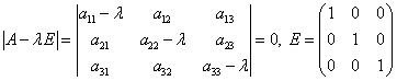
This equation is a third order algebraic equation, therefore it has 3 roots. The following cases are possible:
1. The roots (eigenvalues) are real and distinct.
2. Among the roots (eigenvalues) there are complex conjugate ones, let
- real root
=
3. The roots (eigenvalues) are real. One of the roots is a multiple.
To figure out how to act in each of these cases, we will need:
Theorem 1.
Let be the pairwise distinct eigenvalues of matrix A, and let be their corresponding eigenvectors. Then
form a fundamental system of solutions to the original system.
Comment
.
Let be the real eigenvalue of matrix A (the real root of the characteristic equation), and let be the corresponding eigenvector.
= - complex eigenvalues of matrix A, - corresponding - eigenvector. Then
(Re is the real part, Im is the imaginary part)
form a fundamental system of solutions to the original system. (i.e. and = considered together)
Theorem 3.
Let be the root of the characteristic equation of multiplicity 2. Then the original system has 2 linearly independent solutions of the form ![]() ,
,
where , are vector constants. If the multiplicity is 3, then there are 3 linearly independent solutions of the form
.
Vectors are found by substituting solutions (*) and (**) into the original system.
To better understand the method for finding solutions of the form (*) and (**), see the typical examples below.
Now let's look at each of the above cases in more detail.
1. Algorithm for solving homogeneous systems of third-order differential equations in the case of different real roots of the characteristic equation.
Given the system
1) We compose a characteristic equation
- real and distinct eigenvalues of the 9roots of this equation).
2) We build where 
3) We build where
- eigenvector of matrix A, corresponding to , i.e. - any system solution 
4) We build where
- eigenvector of matrix A, corresponding to , i.e. - any system solution 
5)
constitute a fundamental system of solutions. Next we write the general solution of the original system in the form
,
here C 1, C 2, C 3 are arbitrary constants,
,
or in coordinate form 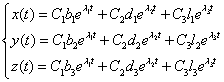
Let's look at a few examples:
Example 1.![]()

2) Find 
3) We find 
4) Vector functions ![]()
![]()
or in coordinate notation 
Example 2.
1) We compose and solve the characteristic equation: 
2) Find 
3) We find 
4) Find 
5) Vector functions 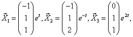
form a fundamental system. The general solution has the form 
or in coordinate notation 
2. Algorithm for solving homogeneous systems of third-order differential equations in the case of complex conjugate roots of the characteristic equation.
- real root,
2) We build where
3) We build
| - eigenvector of matrix A, corresponding to , i.e. satisfies the system |
Here Re is the real part
Im - imaginary part
4) constitute a fundamental system of solutions. Next we write down the general solution of the original system:
, Where
C 1, C 2, C 3 are arbitrary constants.
Example 1.
1) Compose and solve the characteristic equation 
2)We are building

3) We build
, Where

Let's reduce the first equation by 2. Then add the first equation multiplied by 2i to the second equation, and subtract the first one multiplied by 2 from the third equation. 
Next 
Hence, 
4) - fundamental system of solutions. Let us write down the general solution of the original system: 
Example 2.![]()
1) We compose and solve the characteristic equation 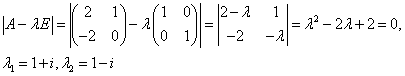
2)We are building
(i.e., and considered together), where

Multiply the second equation by (1-i) and reduce by 2. 

Hence, ![]()
3)
General solution of the original system
or 
2. Algorithm for solving homogeneous systems of third-order differential equations in the case of multiple roots of the characteristic equation.
We compose and solve the characteristic equation
There are two possible cases: ![]()
Consider case a) 1), where
| - eigenvector of matrix A, corresponding to , i.e. satisfies the system |
2) Let us refer to Theorem 3, from which it follows that there are two linearly independent solutions of the form ![]() ,
,
where , are constant vectors. Let's take them for .
3) - fundamental system of solutions. Next we write down the general solution of the original system:
Consider case b):
1) Let us refer to Theorem 3, from which it follows that there are three linearly independent solutions of the form
,
where , , are constant vectors. Let's take them for .
2) - fundamental system of solutions. Next we write down the general solution of the original system.
To better understand how to find solutions of the form (*), consider several typical examples.
Example 1.
We compose and solve the characteristic equation: 
We have case a)
1) We build  , Where

From the second equation we subtract the first:
 ? The third line is similar to the second, we cross it out. Subtract the second from the first equation:
2) = 1 (multiples of 2)
According to T.3, this root must correspond to two linearly independent solutions of the form .
Let's try to find all linearly independent solutions for which, i.e. solutions of the form
.
Such a vector will be a solution if and only if is the eigenvector corresponding to =1, i.e.
, or  , the second and third lines are similar to the first, throw them out.
 ![]()
The system has been reduced to one equation. Consequently, there are two free unknowns, for example, and . Let's first give them the values 1, 0; then the values 0, 1. We get the following solutions:  .
.
Hence,  .
.
3) - fundamental system of solutions. It remains to write down the general solution of the original system: 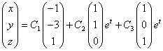 . .. Thus, there is only one solution of the form Let's substitute X 3 into this system: Cross out the third line (it is similar to the second). The system is consistent (has a solution) for any c. Let c=1.
or