What is mathematical expectation in simple terms. Mathematical expectation (Population mean) is. Dependence on the number of experiments

– the number of boys among 10 newborns.

It is absolutely clear that this number is not known in advance, and the next ten children born may include:

Or boys - one and only one from the listed options.

And, in order to keep in shape, a little physical education:

– long jump distance (in some units).

Even a master of sports cannot predict it :)

However, your hypotheses?

2) Continuous random variable – accepts All numerical values ​​from some finite or infinite interval.

Note : V educational literature popular abbreviations DSV and NSV

First, let's analyze the discrete random variable, then - continuous.

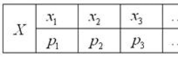
Distribution law of a discrete random variable

- This correspondence between possible values ​​of this quantity and their probabilities. Most often, the law is written in a table:

The term is used quite often row distribution, but in some situations it sounds ambiguous, and so I will stick to the "law".

And now very important point: since the random variable Necessarily will accept one of the values, then the corresponding events form full group and the sum of the probabilities of their occurrence is equal to one:

or, if written condensed:

So, for example, the law of probability distribution of points rolled on a die has the following form:

No comments.

You may be under the impression that a discrete random variable can only take on “good” integer values. Let's dispel the illusion - they can be anything:

Example 1

Some game has the following winning distribution law:

...you've probably dreamed of such tasks for a long time :) I'll tell you a secret - me too. Especially after finishing work on field theory.

Solution: since a random variable can take only one of three values, the corresponding events form full group, which means the sum of their probabilities is equal to one:

Exposing the “partisan”:

– thus, the probability of winning conventional units is 0.4.

Control: that’s what we needed to make sure of.

Answer:

It is not uncommon when you need to create a distribution law yourself. For this they use classical definition of probability, multiplication/addition theorems for event probabilities and other chips tervera:

Example 2

The box contains 50 lottery tickets, among which there are 12 winning ones, and 2 of them win 1000 rubles each, and the rest - 100 rubles each. Create a distribution law random variable– the size of the winnings if one ticket is drawn at random from the box.

Solution: as you noticed, the values ​​of a random variable are usually placed in in ascending order. Therefore, we start with the smallest winnings, namely rubles.

There are 50 such tickets in total - 12 = 38, and according to classical definition:
– the probability that a randomly drawn ticket will be a loser.

In other cases everything is simple. The probability of winning rubles is:

Check: – and this is a particularly pleasant moment of such tasks!

Answer: the desired law of distribution of winnings:

Next task for independent decision:

Example 3

The probability that the shooter will hit the target is . Draw up a distribution law for a random variable - the number of hits after 2 shots.

...I knew that you missed him :) Let's remember multiplication and addition theorems. The solution and answer are at the end of the lesson.

The distribution law completely describes a random variable, but in practice it can be useful (and sometimes more useful) to know only some of it numerical characteristics .

Expectation of a discrete random variable

Speaking in simple language, This average expected value when testing is repeated many times. Let the random variable take values ​​with probabilities respectively. Then mathematical expectation of this random variable is equal to sum of products all its values ​​to the corresponding probabilities:

or collapsed:

Let us calculate, for example, the mathematical expectation of a random variable - the number of points rolled on a die:

Now let's remember our hypothetical game:

The question arises: is it profitable to play this game at all? ...who has any impressions? So you can’t say it “offhand”! But this question can be easily answered by calculating the mathematical expectation, essentially - weighted average by probability of winning:

Thus, the mathematical expectation of this game losing.

Don't trust your impressions - trust the numbers!

Yes, here you can win 10 and even 20-30 times in a row, but in the long run we will face inevitable ruin. And I wouldn't advise you to play such games :) Well, maybe only for fun.

From all of the above it follows that the mathematical expectation is no longer a RANDOM value.

Creative task for independent research:

Example 4

Mr. X plays European roulette using the following system: he constantly bets 100 rubles on “red”. Draw up a law of distribution of a random variable - its winnings. Calculate the mathematical expectation of winnings and round it to the nearest kopeck. How many on average Does the player lose for every hundred he bet?

Reference : European roulette contains 18 red, 18 black and 1 green sector (“zero”). If “red” is rolled out, the player is paid double the bet, otherwise it goes to the casino’s income

There are many other roulette systems for which you can create your own probability tables. But this is the case when we do not need any distribution laws and tables, because it has been established for certain that the player’s mathematical expectation will be exactly the same. The only thing that changes from system to system is

Mathematical expectation- the average value of a random variable (probability distribution of a stationary random variable) when the number of samples or the number of measurements (sometimes called the number of tests) tends to infinity.

Arithmetic mean of a one-dimensional random variable finite number tests are usually called mathematical expectation estimate. As the number of trials of a stationary random process tends to infinity, the estimate of the mathematical expectation tends to the mathematical expectation.

Mathematical expectation is one of the basic concepts in probability theory).

Encyclopedic YouTube

1 / 5

✪ Expectation and variance - bezbotvy

✪ Probability Theory 15: Expectation

✪ Mathematical expectation

✪ Expectation and variance. Theory

✪ Mathematical expectation in trading

Subtitles

Definition

Let a probability space be given (Ω , A , P) (\displaystyle (\Omega ,(\mathfrak (A)),\mathbb (P))) and a random variable defined on it X (\displaystyle X). That is, by definition, X: Ω → R (\displaystyle X\colon \Omega \to \mathbb (R) )- measurable function. If there exists a Lebesgue integral of X (\displaystyle X) by space Ω (\displaystyle \Omega ), then it is called the mathematical expectation, or the average (expected) value and is denoted M [ X ] (\displaystyle M[X]) or E [ X ] (\displaystyle \mathbb (E) [X]).

M [ X ] = ∫ Ω X (ω) P (d ω) . (\displaystyle M[X]=\int \limits _(\Omega )\!X(\omega)\,\mathbb (P) (d\omega).)

Basic formulas for mathematical expectation

M [ X ] = ∫ − ∞ ∞ x d F X (x) ; x ∈ R (\displaystyle M[X]=\int \limits _(-\infty )^(\infty )\!x\,dF_(X)(x);x\in \mathbb (R) ).

Mathematical expectation of a discrete distribution

P (X = x i) = p i , ∑ i = 1 ∞ p i = 1 (\displaystyle \mathbb (P) (X=x_(i))=p_(i),\;\sum \limits _(i=1 )^(\infty )p_(i)=1),

then it follows directly from the definition of the Lebesgue integral that

M [ X ] = ∑ i = 1 ∞ x i p i (\displaystyle M[X]=\sum \limits _(i=1)^(\infty )x_(i)\,p_(i)).

Expectation of an integer value

P (X = j) = p j , j = 0 , 1 , . . . ; ∑ j = 0 ∞ p j = 1 (\displaystyle \mathbb (P) (X=j)=p_(j),\;j=0,1,...;\quad \sum \limits _(j=0 )^(\infty )p_(j)=1)

then its mathematical expectation can be expressed through the generating function of the sequence ( p i ) (\displaystyle \(p_(i)\))

P (s) = ∑ k = 0 ∞ p k s k (\displaystyle P(s)=\sum _(k=0)^(\infty )\;p_(k)s^(k))

as the value of the first derivative in unity: M [ X ] = P ′ (1) (\displaystyle M[X]=P"(1)). If the mathematical expectation X (\displaystyle X) infinitely, then lim s → 1 P ′ (s) = ∞ (\displaystyle \lim _(s\to 1)P"(s)=\infty ) and we will write P ′ (1) = M [ X ] = ∞ (\displaystyle P"(1)=M[X]=\infty )

Now let's take the generating function Q (s) (\displaystyle Q(s)) sequences of distribution tails ( q k ) (\displaystyle \(q_(k)\))

q k = P (X > k) = ∑ j = k + 1 ∞ p j ; Q (s) = ∑ k = 0 ∞ q k s k . (\displaystyle q_(k)=\mathbb (P) (X>k)=\sum _(j=k+1)^(\infty )(p_(j));\quad Q(s)=\sum _(k=0)^(\infty )\;q_(k)s^(k).)

This generating function is related to the previously defined function P(s) (\displaystyle P(s)) property: Q (s) = 1 − P (s) 1 − s (\displaystyle Q(s)=(\frac (1-P(s))(1-s))) at | s |< 1 {\displaystyle |s|<1} . From this, by the mean value theorem, it follows that the mathematical expectation is simply equal to the value of this function in unity:

M [ X ] = P ′ (1) = Q (1) (\displaystyle M[X]=P"(1)=Q(1))

Mathematical expectation of an absolutely continuous distribution

M [ X ] = ∫ − ∞ ∞ x f X (x) d x (\displaystyle M[X]=\int \limits _(-\infty )^(\infty )\!xf_(X)(x)\,dx ).

Mathematical expectation of a random vector

Let X = (X 1 , … , X n) ⊤ : Ω → R n (\displaystyle X=(X_(1),\dots ,X_(n))^(\top )\colon \Omega \to \mathbb ( R)^(n))- random vector. Then by definition

M [ X ] = (M [ X 1 ] , … , M [ X n ]) ⊤ (\displaystyle M[X]=(M,\dots ,M)^(\top )),

that is, the mathematical expectation of a vector is determined component by component.

Expectation of transformation of a random variable

Let g: R → R (\displaystyle g\colon \mathbb (R) \to \mathbb (R) ) is a Borel function such that the random variable Y = g (X) (\displaystyle Y=g(X)) has a finite mathematical expectation. Then the formula is valid for it

M [ g (X) ] = ∑ i = 1 ∞ g (x i) p i , (\displaystyle M\left=\sum \limits _(i=1)^(\infty )g(x_(i))p_( i),)

If X (\displaystyle X) has a discrete distribution;

M [ g (X) ] = ∫ − ∞ ∞ g (x) f X (x) d x , (\displaystyle M\left=\int \limits _(-\infty )^(\infty )\!g(x )f_(X)(x)\,dx,)

If X (\displaystyle X) has an absolutely continuous distribution.

If the distribution P X (\displaystyle \mathbb (P) ^(X)) random variable X (\displaystyle X) general view, then

M [ g (X) ] = ∫ − ∞ ∞ g (x) P X (d x) . (\displaystyle M\left=\int \limits _(-\infty )^(\infty )\!g(x)\,\mathbb (P) ^(X)(dx).)

In the special case when g (X) = X k (\displaystyle g(X)=X^(k)), mathematical expectation M [ g (X) ] = M [ X k ] (\displaystyle M=M) called k (\displaystyle k)-m moment of the random variable.

The simplest properties of mathematical expectation

• The mathematical expectation of a number is the number itself.

M [ a ] ​​= a (\displaystyle M[a]=a) a ∈ R (\displaystyle a\in \mathbb (R) )- constant;

• The mathematical expectation is linear, that is

M [ a X + b Y ] = a M [ X ] + b M [ Y ] (\displaystyle M=aM[X]+bM[Y]), Where X , Y (\displaystyle X,Y) are random variables with finite mathematical expectation, and a , b ∈ R (\displaystyle a,b\in \mathbb (R) )- arbitrary constants; 0 ⩽ M [ X ] ⩽ M [ Y ] (\displaystyle 0\leqslant M[X]\leqslant M[Y]); M [ X ] = M [ Y ] (\displaystyle M[X]=M[Y]). M [ X Y ] = M [ X ] M [ Y ] (\displaystyle M=M[X]M[Y]).

The mathematical expectation (average value) of a random variable X given on a discrete probability space is the number m =M[X]=∑x i p i if the series converges absolutely.

Purpose of the service. Using the online service mathematical expectation, variance and standard deviation are calculated(see example). In addition, a graph of the distribution function F(X) is plotted.

Properties of the mathematical expectation of a random variable

1. The mathematical expectation of a constant value is equal to itself: M[C]=C, C – constant;
2. M=C M[X]
3. The mathematical expectation of the sum of random variables is equal to the sum of their mathematical expectations: M=M[X]+M[Y]
4. The mathematical expectation of the product of independent random variables is equal to the product of their mathematical expectations: M=M[X] M[Y] , if X and Y are independent.

Dispersion properties

1. The variance of a constant value is zero: D(c)=0.
2. The constant factor can be taken out from under the dispersion sign by squaring it: D(k*X)= k 2 D(X).
3. If the random variables X and Y are independent, then the variance of the sum is equal to the sum of the variances: D(X+Y)=D(X)+D(Y).
4. If random variables X and Y are dependent: D(X+Y)=DX+DY+2(X-M[X])(Y-M[Y])
5. The following computational formula is valid for dispersion:
   D(X)=M(X 2)-(M(X)) 2

Example. The mathematical expectations and variances of two independent random variables X and Y are known: M(x)=8, M(Y)=7, D(X)=9, D(Y)=6. Find the mathematical expectation and variance of the random variable Z=9X-8Y+7.
Solution. Based on the properties of mathematical expectation: M(Z) = M(9X-8Y+7) = 9*M(X) - 8*M(Y) + M(7) = 9*8 - 8*7 + 7 = 23 .
Based on the properties of dispersion: D(Z) = D(9X-8Y+7) = D(9X) - D(8Y) + D(7) = 9^2D(X) - 8^2D(Y) + 0 = 81*9 - 64*6 = 345

Algorithm for calculating mathematical expectation

Properties of discrete random variables: all their values ​​can be renumbered by natural numbers; Assign each value a non-zero probability.

1. We multiply the pairs one by one: x i by p i .
2. Add the product of each pair x i p i .
   For example, for n = 4: m = ∑x i p i = x 1 p 1 + x 2 p 2 + x 3 p 3 + x 4 p 4

Distribution function of a discrete random variable stepwise, it increases abruptly at those points whose probabilities are positive.

Example No. 1.

x i	1	3	4	7	9
p i	0.1	0.2	0.1	0.3	0.3

We find the mathematical expectation using the formula m = ∑x i p i .
Expectation M[X].
M[x] = 1*0.1 + 3*0.2 + 4*0.1 + 7*0.3 + 9*0.3 = 5.9
We find the variance using the formula d = ∑x 2 i p i - M[x] 2 .
Variance D[X].
D[X] = 1 2 *0.1 + 3 2 *0.2 + 4 2 *0.1 + 7 2 *0.3 + 9 2 *0.3 - 5.9 2 = 7.69
Standard deviation σ(x).
σ = sqrt(D[X]) = sqrt(7.69) = 2.78

Example No. 2. A discrete random variable has the following distribution series:

X	-10	-5	0	5	10
r	A	0,32	2a	0,41	0,03

Find the value of a, the mathematical expectation and the standard deviation of this random variable.

Solution. The value of a is found from the relation: Σp i = 1
Σp i = a + 0.32 + 2 a + 0.41 + 0.03 = 0.76 + 3 a = 1
0.76 + 3 a = 1 or 0.24=3 a , from where a = 0.08

Example No. 3. Determine the distribution law of a discrete random variable if its variance is known, and x 1 x 1 =6; x 2 =9; x 3 =x; x 4 =15
p 1 =0.3; p 2 =0.3; p 3 =0.1; p 4 =0.3
d(x)=12.96

Solution.
Here you need to create a formula for finding the variance d(x):
d(x) = x 1 2 p 1 +x 2 2 p 2 +x 3 2 p 3 +x 4 2 p 4 -m(x) 2
where expectation m(x)=x 1 p 1 +x 2 p 2 +x 3 p 3 +x 4 p 4
For our data
m(x)=6*0.3+9*0.3+x 3 *0.1+15*0.3=9+0.1x 3
12.96 = 6 2 0.3+9 2 0.3+x 3 2 0.1+15 2 0.3-(9+0.1x 3) 2
or -9/100 (x 2 -20x+96)=0
Accordingly, we need to find the roots of the equation, and there will be two of them.
x 3 =8, x 3 =12
Choose the one that satisfies the condition x 1 x 3 =12

Distribution law of a discrete random variable
x 1 =6; x 2 =9; x 3 =12; x 4 =15
p 1 =0.3; p 2 =0.3; p 3 =0.1; p 4 =0.3

The mathematical expectation of a discrete random variable is the sum of the products of all its possible values ​​and their probabilities.

Let a random variable take only probability values ​​which are respectively equal. Then the mathematical expectation of a random variable is determined by the equality

If a discrete random variable takes a countable set of possible values, then

Moreover, the mathematical expectation exists if the series on the right side of the equality converges absolutely.

Comment. From the definition it follows that the mathematical expectation of a discrete random variable is a non-random (constant) quantity.

Definition of mathematical expectation in the general case

Let us determine the mathematical expectation of a random variable whose distribution is not necessarily discrete. Let's start with the case of non-negative random variables. The idea will be to approximate such random variables using discrete ones for which the mathematical expectation has already been determined, and set the mathematical expectation equal to the limit of the mathematical expectations of the discrete random variables that approximate it. By the way, this is a very useful general idea, which is that some characteristic is first determined for simple objects, and then for more complex objects it is determined by approximating them by simpler ones.

Lemma 1. Let there be an arbitrary non-negative random variable. Then there is a sequence of discrete random variables such that

Proof. Let us divide the semi-axis into equal length segments and determine

Then properties 1 and 2 easily follow from the definition of a random variable, and

Lemma 2. Let be a non-negative random variable and and two sequences of discrete random variables possessing properties 1-3 from Lemma 1. Then

Proof. Note that for non-negative random variables we allow

By virtue of Property 3, it is easy to see that there is a sequence of positive numbers such that

It follows that

Using the properties of mathematical expectations for discrete random variables, we obtain

Passing to the limit at we obtain the statement of Lemma 2.

Definition 1. Let be a non-negative random variable, - a sequence of discrete random variables that have properties 1-3 from Lemma 1. The mathematical expectation of a random variable is the number

Lemma 2 guarantees that it does not depend on the choice of approximating sequence.

Let now be an arbitrary random variable. Let's define

From the definition and it easily follows that

Definition 2. The mathematical expectation of an arbitrary random variable is the number

If at least one of the numbers on the right side of this equality is finite.

Properties of mathematical expectation

Property 1. The mathematical expectation of a constant value is equal to the constant itself:

Proof. We will consider a constant as a discrete random variable that has one possible value and takes it with probability, therefore,

Remark 1. Let us define the product of a constant variable by a discrete random variable as a discrete random whose possible values ​​are equal to the products of the constant by the possible values; the probabilities of possible values ​​are equal to the probabilities of the corresponding possible values. For example, if the probability of a possible value is equal then the probability that the value will take the value is also equal

Property 2. The constant factor can be taken out of the sign of the mathematical expectation:

Proof. Let the random variable be given by the probability distribution law:

Taking into account Remark 1, we write the distribution law of the random variable

Remark 2. Before moving on to the next property, we point out that two random variables are called independent if the distribution law of one of them does not depend on what possible values ​​the other variable took. Otherwise, the random variables are dependent. Several random variables are called mutually independent if the laws of distribution of any number of them do not depend on what possible values ​​the remaining variables took.

Remark 3. Let us define the product of independent random variables and as a random variable whose possible values ​​are equal to the products of each possible value by each possible value, the probabilities of the possible values ​​of the product are equal to the products of the probabilities of the possible values ​​of the factors. For example, if the probability of a possible value is, the probability of a possible value is then the probability of a possible value is

Property 3. The mathematical expectation of the product of two independent random variables is equal to the product of their mathematical expectations:

Proof. Let independent random variables be specified by their own probability distribution laws:

Let's compile all the values ​​that a random variable can take. To do this, let's multiply all possible values ​​by each possible value; As a result, we obtain and, taking into account Remark 3, we write the distribution law, assuming for simplicity that all possible values ​​of the product are different (if this is not the case, then the proof is carried out in a similar way):

The mathematical expectation is equal to the sum of the products of all possible values ​​and their probabilities:

Consequence. The mathematical expectation of the product of several mutually independent random variables is equal to the product of their mathematical expectations.

Property 4. The mathematical expectation of the sum of two random variables is equal to the sum of the mathematical expectations of the terms:

Proof. Let random variables and be specified by the following distribution laws:

Let's compile all possible values ​​of a quantity. To do this, we add each possible value to each possible value; we obtain. Let us assume for simplicity that these possible values ​​are different (if this is not the case, then the proof is carried out in a similar way), and we denote their probabilities respectively by and

The mathematical expectation of a value is equal to the sum of the products of possible values ​​and their probabilities:

Let us prove that an Event that will take on the value (the probability of this event is equal) entails an event that will take on the value or (the probability of this event by the addition theorem is equal), and vice versa. Hence it follows that the equalities are proved similarly

Substituting the right-hand sides of these equalities into relation (*), we obtain

or finally

Variance and standard deviation

In practice, it is often necessary to estimate the dispersion of possible values ​​of a random variable around its mean value. For example, in artillery it is important to know how closely the shells will fall near the target that is to be hit.

At first glance, it may seem that the easiest way to estimate dispersion is to calculate all possible deviations of a random variable and then find their average value. However, this path will not give anything, since the average value of the deviation, i.e. for any random variable is equal to zero. This property is explained by the fact that some possible deviations are positive, while others are negative; as a result of their mutual cancellation, the average deviation value is zero. These considerations indicate the advisability of replacing possible deviations with their absolute values ​​or their squares. This is what they do in practice. True, in the case when possible deviations are replaced by absolute values, one has to operate with absolute values, which sometimes leads to serious difficulties. Therefore, most often they take a different path, i.e. calculate the average value of the squared deviation, which is called dispersion.

In the previous one, we presented a number of formulas that allow us to find the numerical characteristics of functions when the laws of distribution of arguments are known. However, in many cases, to find the numerical characteristics of functions, it is not necessary to even know the laws of distribution of arguments, but it is enough to know only some of their numerical characteristics; at the same time, we generally do without any laws of distribution. Determining the numerical characteristics of functions from given numerical characteristics of arguments is widely used in probability theory and can significantly simplify the solution of a number of problems. Most of these simplified methods relate to linear functions; however, some elementary nonlinear functions also allow a similar approach.

In the present we will present a number of theorems on the numerical characteristics of functions, which together represent a very simple apparatus for calculating these characteristics, applicable in a wide range of conditions.

1. Mathematical expectation of a non-random value

The formulated property is quite obvious; it can be proven by considering a non-random variable as a special type of random, with one possible value with probability one; then according to the general formula for the mathematical expectation:

.

2. Variance of a non-random quantity

If is a non-random value, then

3. Substituting a non-random value for the sign of mathematical expectation

, (10.2.1)

that is, a non-random value can be taken out as a sign of the mathematical expectation.

Proof.

a) For discontinuous quantities

b) For continuous quantities

.

4. Taking a non-random value out of the sign of dispersion and standard deviation

If is a non-random quantity, and is random, then

, (10.2.2)

that is, a non-random value can be taken out of the sign of the dispersion by squaring it.

Proof. By definition of variance

Consequence

,

that is, a non-random value can be taken out of the sign of the standard deviation by its absolute value. We obtain the proof by taking the square root from formula (10.2.2) and taking into account that the r.s.o. - a significantly positive value.

5. Mathematical expectation of the sum of random variables

Let us prove that for any two random variables and

that is, the mathematical expectation of the sum of two random variables is equal to the sum of their mathematical expectations.

This property is known as the theorem of addition of mathematical expectations.

Proof.

a) Let be a system of discontinuous random variables. Let us apply the general formula (10.1.6) to the sum of random variables for the mathematical expectation of a function of two arguments:

.

Ho represents nothing more than the total probability that the quantity will take the value :

;

hence,

.

We will similarly prove that

,

and the theorem is proven.

b) Let be a system of continuous random variables. According to formula (10.1.7)

. (10.2.4)

Let us transform the first of the integrals (10.2.4):

;

similarly

,

and the theorem is proven.

It should be specially noted that the theorem for adding mathematical expectations is valid for any random variables - both dependent and independent.

The theorem for adding mathematical expectations is generalized to an arbitrary number of terms:

, (10.2.5)

that is, the mathematical expectation of the sum of several random variables is equal to the sum of their mathematical expectations.

To prove it, it is enough to use the method of complete induction.

6. Mathematical expectation of a linear function

Consider a linear function of several random arguments:

where are non-random coefficients. Let's prove that

, (10.2.6)

i.e. the mathematical expectation of a linear function is equal to the same linear function of the mathematical expectations of the arguments.

Proof. Using the addition theorem of m.o. and the rule of placing a non-random quantity outside the sign of the m.o., we obtain:

.

7. Dispepthis sum of random variables

The variance of the sum of two random variables is equal to the sum of their variances plus twice the correlation moment:

Proof. Let's denote

According to the theorem of addition of mathematical expectations

Let's move from random variables to the corresponding centered variables. Subtracting equality (10.2.9) term by term from equality (10.2.8), we have:

By definition of variance

Q.E.D.

Formula (10.2.7) for the variance of the sum can be generalized to any number of terms:

, (10.2.10)

where is the correlation moment of the quantities, the sign under the sum means that the summation extends to all possible pairwise combinations of random variables .

The proof is similar to the previous one and follows from the formula for the square of a polynomial.

Formula (10.2.10) can be written in another form:

, (10.2.11)

where the double sum extends to all elements of the correlation matrix of the system of quantities , containing both correlation moments and variances.

If all random variables , included in the system, are uncorrelated (i.e., when ), formula (10.2.10) takes the form:

, (10.2.12)

that is, the variance of the sum of uncorrelated random variables is equal to the sum of the variances of the terms.

This position is known as the theorem of addition of variances.

8. Variance of a linear function

Let's consider a linear function of several random variables.

where are non-random quantities.

Let us prove that the dispersion of this linear function is expressed by the formula

, (10.2.13)

where is the correlation moment of the quantities , .

Proof. Let us introduce the notation:

. (10.2.14)

Applying formula (10.2.10) for the dispersion of the sum to the right side of expression (10.2.14) and taking into account that , we obtain:

where is the correlation moment of the quantities:

.

Let's calculate this moment. We have:

;

similarly

Substituting this expression into (10.2.15), we arrive at formula (10.2.13).

In the special case when all quantities are uncorrelated, formula (10.2.13) takes the form:

, (10.2.16)

that is, the variance of a linear function of uncorrelated random variables is equal to the sum of the products of the squares of the coefficients and the variances of the corresponding arguments.

9. Mathematical expectation of a product of random variables

The mathematical expectation of the product of two random variables is equal to the product of their mathematical expectations plus the correlation moment:

Proof. We will proceed from the definition of the correlation moment:

Let's transform this expression using the properties of mathematical expectation:

which is obviously equivalent to formula (10.2.17).

If random variables are uncorrelated, then formula (10.2.17) takes the form:

that is, the mathematical expectation of the product of two uncorrelated random variables is equal to the product of their mathematical expectations.

This position is known as the theorem of multiplication of mathematical expectations.

Formula (10.2.17) is nothing more than an expression of the second mixed central moment of the system through the second mixed initial moment and mathematical expectations:

. (10.2.19)

This expression is often used in practice when calculating the correlation moment in the same way that for one random variable the variance is often calculated through the second initial moment and the mathematical expectation.

The theorem of multiplication of mathematical expectations is generalized to an arbitrary number of factors, only in this case, for its application, it is not enough that the quantities are uncorrelated, but it is required that some higher mixed moments, the number of which depends on the number of terms in the product, vanish. These conditions are certainly satisfied if the random variables included in the product are independent. In this case

, (10.2.20)

that is, the mathematical expectation of the product of independent random variables is equal to the product of their mathematical expectations.

This proposition can be easily proven by complete induction.

10. Variance of the product of independent random variables

Let us prove that for independent quantities

Proof. Let's denote . By definition of variance

Since the quantities are independent, and

When independent, the quantities are also independent; hence,

,

But there is nothing more than the second initial moment of the magnitude, and, therefore, is expressed through the dispersion:

;

similarly

.

Substituting these expressions into formula (10.2.22) and bringing similar terms, we arrive at formula (10.2.21).

In the case when centered random variables (variables with mathematical expectations equal to zero) are multiplied, formula (10.2.21) takes the form:

, (10.2.23)

that is, the variance of the product of independent centered random variables is equal to the product of their variances.

11. Higher moments of the sum of random variables

In some cases it is necessary to calculate the highest moments of the sum of independent random variables. Let us prove some relations related here.

1) If the quantities are independent, then

Proof.

whence, according to the theorem of multiplication of mathematical expectations

But the first central moment for any quantity is zero; the two middle terms vanish, and formula (10.2.24) is proven.

Relation (10.2.24) is easily generalized by induction to an arbitrary number of independent terms:

. (10.2.25)

2) The fourth central moment of the sum of two independent random variables is expressed by the formula

where are the variances of the quantities and .

The proof is completely similar to the previous one.

Using the method of complete induction, it is easy to prove the generalization of formula (10.2.26) to an arbitrary number of independent terms.