Class: 10
Presentation for the lesson


 Back forward
Attention! Slide previews are for informational purposes only and may not represent all the features of the presentation. If you are interested in this work, please download the full version.
Lesson objectives: Study the state of balance of bodies, get acquainted with different types of balance; find out the conditions under which the body is in equilibrium.
Lesson objectives:
- Educational: Study two conditions of equilibrium, types of equilibrium (stable, unstable, indifferent). Find out under what conditions bodies are more stable.
- Educational: To promote the development of cognitive interest in physics. Development of skills to compare, generalize, highlight the main thing, draw conclusions.
- Educational: Cultivate attention, the ability to express one’s point of view and defend it, develop communication skills students.
Lesson type: lesson on learning new material with computer support.
Equipment:
- Disc “Work and Power” from “Electronic Lessons and Tests.
- Table "Equilibrium conditions".
- Tilting prism with plumb line.
- Geometric bodies: cylinder, cube, cone, etc.
- Computer, multimedia projector, interactive whiteboard or screen.
- Presentation.
During the classes
Today in the lesson we will learn why the crane does not fall, why the Vanka-Vstanka toy always returns to its original state, why the Leaning Tower of Pisa does not fall?
I. Repetition and updating of knowledge.
- State Newton's first law. What condition does the law refer to?
- What question does Newton's second law answer? Formula and formulation.
- What question does Newton's third law answer? Formula and formulation.
- What is the resultant force? How is she located?
- From the disk “Motion and interaction of bodies” complete task No. 9 “Resultant of forces with different directions” (the rule for adding vectors (2, 3 exercises)).
II. Learning new material.
1. What is called equilibrium?
Balance is a state of rest.
2. Equilibrium conditions.(slide 2)
a) When is the body at rest? What law does this follow from?
First equilibrium condition: A body is in equilibrium if the geometric sum external forces, applied to the body, is equal to zero. ∑F = 0
b) Let two act on the board equal forces, as it shown on the picture.

Will it be in balance? (No, she will turn)
Only the central point is at rest, the rest are moving. This means that for a body to be in equilibrium, it is necessary that the sum of all forces acting on each element equals 0.
Second equilibrium condition: The sum of the moments of forces acting clockwise must be equal to the sum of the moments of forces acting counterclockwise.
∑ M clockwise = ∑ M counterclockwise
Moment of force: M = F L
L – arm of force – the shortest distance from the fulcrum to the line of action of the force.
3. The center of gravity of the body and its location.(slide 4)
Body center of gravity- this is the point through which the resultant of all parallel forces of gravity acting on individual elements of the body passes (for any position of the body in space).
Find the center of gravity of the following figures:

4. Types of balance.
A) (slides 5–8)


Conclusion: Equilibrium is stable if, with a small deviation from the equilibrium position, there is a force tending to return it to this position.
The position in which it is potential energy minimal. (slide 9)
b) Stability of bodies located at the point of support or on the line of support.(slides 10–17)

Conclusion: For the stability of a body located at one point or line of support, it is necessary that the center of gravity be below the point (line) of support.
c) Stability of bodies located on a flat surface.
(slide 18)
1) Support surface– this is not always the surface that is in contact with the body (but the one that is limited by the lines connecting the legs of the table, tripod)

2) Analysis of the slide from “Electronic lessons and tests”, disk “Work and power”, lesson “Types of balance”.
Picture 1.
- How are the stools different? (Support area)
- Which one is more stable? (With larger area)
- How are the stools different? (Location of the center of gravity)
- Which one is the most stable? (Which center of gravity is lower)
- Why? (Because it can be tilted to a larger angle without tipping over)
3) Experiment with a deflecting prism
- Let's put a prism with a plumb line on the board and begin to gradually lift it by one edge. What do we see?
- As long as the plumb line intersects the surface bounded by the support, equilibrium is maintained. But as soon as the vertical line passing through the center of gravity begins to go beyond the boundaries of the support surface, the whatnot tips over.
Parsing slides 19–22.

Conclusions:
- The body that has the largest support area is stable.
- Of two bodies of the same area, the one whose center of gravity is lower is stable, because it can be tilted without tipping over at a large angle.
Parsing slides 23–25.

Which ships are the most stable? Why? (In which the cargo is located in the holds, and not on the deck)

Which cars are the most stable? Why? (To increase the stability of cars when turning, the road surface is tilted in the direction of the turn.)
Conclusions: Equilibrium can be stable, unstable, indifferent. The greater the support area and the lower the center of gravity, the greater the stability of bodies.
III. Application of knowledge about the stability of bodies.
- Which specialties are most in need of knowledge about body balance?
- Designers and constructors of various structures ( high-rise buildings, bridges, television towers, etc.)
- Circus performers.
- Drivers and other professionals.
(slides 28–30)
- Why does “Vanka-Vstanka” return to the equilibrium position at any tilt of the toy?
- Why does the Leaning Tower of Pisa stand at an angle and not fall?
- How do cyclists and motorcyclists maintain balance?
Conclusions from the lesson:
- There are three types of equilibrium: stable, unstable, indifferent.
- A stable position of a body in which its potential energy is minimal.
- The greater the support area and the lower the center of gravity, the greater the stability of bodies on a flat surface.
Homework: § 54 – 56 (G.Ya. Myakishev, B.B. Bukhovtsev, N.N. Sotsky)
Sources and literature used:
- G.Ya. Myakishev, B.B. Bukhovtsev, N.N. Sotsky. Physics. Grade 10.
- Filmstrip “Sustainability” 1976 (scanned by me on a film scanner).
- Disc “Motion and interaction of bodies” from “Electronic lessons and tests”.
- Disc "Work and Power" from "Electronic Lessons and Tests".
Main types of balance points
Let a second order linear homogeneous system with constant coefficients be given: \[\left\( \begin(array)(l) \frac((dx))((dt)) = (a_(11))x + (a_(12 ))y\\ \frac((dy))((dt)) = (a_(21))x + (a_(22))y \end(array) \right..\] This system of equations is autonomous, since the right-hand sides of the equations do not explicitly contain the independent variable \(t.\)
IN matrix form the system of equations is written as \[ (\mathbf(X") = A\mathbf(X),\;\;\text(where)\;\;\mathbf(X) = \left((\begin(array)( *(20)(c)) x\\ y \end(array)) \right),)\;\; (A = \left((\begin(array)(*(20)(c)) (( a_(11)))&((a_(12)))\\ ((a_(21)))&((a_(22))) \end(array)) \right).) \] The equilibrium positions are from the solution of the stationary equation \ This equation has a unique solution \(\mathbf(X) = \mathbf(0),\) if the matrix \(A\) is non-degenerate , i.e. provided \(\det A \ne 0.\) In the case singular matrix the system has an infinite number of equilibrium points.
The classification of equilibrium positions is determined eigenvalues \((\lambda _1),(\lambda _2)\) matrices \(A.\) The numbers \((\lambda _1),(\lambda _2)\) are found from the solution characteristic equation \[(\lambda ^2) - \left(((a_(11)) + (a_(22))) \right)\lambda + (a_(11))(a_(22)) - (a_(12 ))(a_(21)) = 0.\] In the general case, when the matrix \(A\) is non-singular, there are \(4\) different types of equilibrium points:
The stability of equilibrium positions is determined general theorems on stability. Thus, if the real eigenvalues (or the real parts of complex eigenvalues) are negative, then the equilibrium point is asymptotically stable . Examples of such equilibrium positions are steady focus .
If the real part of at least one eigenvalue is positive, then the corresponding equilibrium position is unstable . For example, it could be .
Finally, in the case of purely imaginary roots (the equilibrium point is center) we are dealing with classical stability in the Lyapunov sense .
Our further goal is to study the behavior of solutions near equilibrium positions. For \(2\)-th order systems this is convenient to do graphically using phase portrait , which is a collection phase trajectories on coordinate plane. Arrows on phase trajectories show the direction of movement of a point (i.e., some specific state of the system) over time.
Let us consider in more detail each type of equilibrium point and the corresponding phase portraits.
Stable and unstable node
The eigenvalues \(((\lambda _1),(\lambda _2))\) of points of type "node" satisfy the conditions: \[(\lambda _1),(\lambda _2) \in \Re,\;\;( \lambda _1) \cdot (\lambda _2) > 0.\] The following special cases may arise here.
The roots \(((\lambda _1),(\lambda _2))\) are different \(\left(((\lambda _1) \ne (\lambda _2)) \right)\) and negative \(\left( ((\lambda _1)
Let us construct a schematic phase portrait of such an equilibrium point. Let, for definiteness, \(\left| ((\lambda _1)) \right|
Since both eigenvalues are negative, the solution \(\mathbf(X) = \mathbf(0)\) is asymptotically stable
. This equilibrium position is called stable node
. At \(t \to \infty\) the phase curves tend to the origin \(\mathbf(X) = \mathbf(0).\)
Let us clarify the direction of the phase trajectories. Since \[ (x\left(t \right) = (C_1)(V_(11))(e^((\lambda _1)t)) + (C_2)(V_(12))(e^((\ lambda _2)t)),)\;\; (y\left(t \right) = (C_1)(V_(21))(e^((\lambda _1)t)) + (C_2)(V_(22))(e^((\lambda _2) t)),) \] then the derivative \(\large\frac((dy))((dx))\normalsize\) is equal to \[\frac((dy))((dx)) = \frac((( C_1)(V_(21))(\lambda _1)(e^((\lambda _1)t)) + (C_2)(V_(22))(\lambda _2)(e^((\lambda _2)t ))))(((C_1)(V_(11))(\lambda _1)(e^((\lambda _1)t)) + (C_2)(V_(12))(\lambda _2)(e^ ((\lambda _2)t)))).\] Divide the numerator and denominator by \(((e^((\lambda _1)t))):\) \[\frac((dy))((dx )) = \frac(((C_1)(V_(21))(\lambda _1) + (C_2)(V_(22))(\lambda _2)(e^(\left(((\lambda _2) - (\lambda _1)) \right)t))))(((C_1)(V_(11))(\lambda _1) + (C_2)(V_(12))(\lambda _2)(e^(\ left(((\lambda _2) - (\lambda _1)) \right)t)))).\] In this case \((\lambda _2) - (\lambda _1)
In the case of \((C_1) = 0\), the derivative for any \(t\) is equal to \[\frac((dy))((dx)) = \frac(((V_(22))))((( V_(12)))),\] i.e. the phase trajectory lies on a straight line directed along the eigenvector \((\mathbf(V)_2).\)
Now let us consider the behavior of phase trajectories for \(t \to -\infty.\) Obviously, the coordinates \(x\left(t \right),y\left(t \right)\) tend to infinity, and the derivative \( \large\frac((dy))((dx))\normalsize\) for \((C_2) \ne 0\) takes the following form: \[\frac((dy))((dx)) = \frac (((C_1)(V_(21))(\lambda _1)(e^(\left(((\lambda _1) - (\lambda _2)) \right)t)) + (C_2)(V_(22 ))(\lambda _2)))(((C_1)(V_(11))(\lambda _1)(e^(\left(((\lambda _1) - (\lambda _2)) \right)t) ) + (C_2)(V_(12))(\lambda _2))) = \frac(((V_(22))))(((V_(12)))),\] i.e. phase curves at points at infinity become parallel to the vector \((\mathbf(V)_2).\)
Accordingly, when \((C_2) = 0\) the derivative is equal to \[\frac((dy))((dx)) = \frac(((V_(21))))(((V_(11))) ).\] In this case, the phase trajectory is determined by the direction of the eigenvector \((\mathbf(V)_1).\)
Taking into account the considered properties of phase trajectories, the phase portrait stable node has the form shown schematically in Figure \(1.\)
In a similar way, one can study the behavior of phase trajectories for other types of equilibrium positions. Next, omitting a detailed analysis, we will carry out the main qualitative characteristics of other equilibrium points.
The roots \(((\lambda _1),(\lambda _2))\) are distinct \(\left(((\lambda _1) \ne (\lambda _2)) \right)\) and positive \(\left( ((\lambda _1) > 0, (\lambda _2)) > 0\right).\)
In this case, the point \(\mathbf(X) = \mathbf(0)\) is called unstable node
. Its phase portrait is shown in Figure \(2.\)
Note that in the case of both stable and unstable nodes, the phase trajectories are tangent to a straight line, which is directed along the eigenvector corresponding to the smaller absolute value eigenvalue \(\lambda.\)
Dicritical node
Let the characteristic equation have one zero root of multiplicity \(2,\), i.e. consider the case \((\lambda _1) = (\lambda _2) = (\lambda) \ne 0.\) In this case, the system has a basis of two eigenvectors, i.e. the geometric multiplicity of the eigenvalue \(\lambda\) is equal to \(2.\) In terms linear algebra this means that the dimension of the eigensubspace of the matrix \(A\) is equal to \(2:\) \(\dim \ker A = 2.\) This situation is realized in systems of the form \[ (\frac((dx))(( dt)) = \lambda x,)\;\; (\frac((dy))((dt)) = \lambda y.) \] The direction of the phase trajectories depends on the sign of \(\lambda.\) Here the following two cases are possible:
Case \((\lambda _1) = (\lambda _2) = (\lambda) This equilibrium position is called stable dicritical node (Figure \(3\)) .
Case \((\lambda _1) = (\lambda _2) = (\lambda) > 0.\) This combination of eigenvalues corresponds to unstable dicritical node (Figure \(4\)).
Degenerate node
Let the eigenvalues of the matrix \(A\) again be the same: \((\lambda _1) = (\lambda _2) = (\lambda) \ne 0.\) Unlike the previous case of a dicritical node, we assume that the geometric multiplicity of the eigenvalue values (or in other words, the dimension of the eigensubspace) is now equal to \(1.\) This means that the matrix \(A\) has only one eigenvector \((\mathbf(V)_1).\) The second linearly independent vector, necessary to compose the basis, is defined as the vector \((\mathbf(W)_1),\) attached to \((\mathbf(V)_1).\)
In the case \((\lambda _1) = (\lambda _2) = (\lambda) the equilibrium point is called stable degenerate node (Figure \(5\)).
When \((\lambda _1) = (\lambda _2) = (\lambda) > 0\) the equilibrium position is called unstable degenerate node (Figure \(6\)).
The equilibrium position is under the conditions \[(\lambda _1),(\lambda _2) \in \Re,\;\;(\lambda _1) \cdot (\lambda _2) 0.\) Eigenvalues \((\lambda _1)\) and \((\lambda _2)\) are associated with the corresponding eigenvectors \((\mathbf(V)_1)\) and \((\mathbf(V)_2).\) Lines directed along the eigenvectors vectors \((\mathbf(V)_1),\) \((\mathbf(V)_2),\) are called separatrices . They are asymptotes for the remaining phase trajectories, which have the form of hyperbolas. Each of the separatrices can be associated with a specific direction of movement. If the separatrix is associated with a negative eigenvalue \((\lambda _1) 0,\) i.e. for the separatrix associated with the vector \((\mathbf(V)_2),\) the movement is directed from the origin. The phase portrait of the saddle is shown schematically in Figure \(7.\)
Steady and unstable focus
Let now the eigenvalues \((\lambda _1),(\lambda _2)\) be complex numbers , whose real parts are not equal to zero. If the matrix \(A\) consists of real numbers, then complex roots will be represented in the form complex conjugate numbers: \[(\lambda _(1,2)) = \alpha \pm i\beta .\] Let us find out what form the phase trajectories have in the vicinity of the origin. Let us construct a complex solution \((\mathbf(X)_1)\left(t \right)\) corresponding to the eigenvalue \((\lambda _1) = \alpha + i\beta:\) \[ ((\mathbf(X )_1)\left(t \right) = (e^((\lambda _1)t))(\mathbf(V)_1) ) = ((e^(\left((\alpha + i\beta ) \ right)t))\left((\mathbf(U) + i\mathbf(W)) \right),) \] where \((\mathbf(V)_1) = \mathbf(U) + i\mathbf (W)\) is a complex-valued eigenvector associated with the number \((\lambda _1),\) \(\mathbf(U)\) and \(\mathbf(W)\) are real vector functions. As a result of transformations, we obtain \[ ((\mathbf(X)_1)\left(t \right) = (e^(\alpha t))(e^(i\beta t))\left((\mathbf(U ) + i\mathbf(W)) \right) ) = ((e^(\alpha t))\left((\cos \beta t + i\sin \beta t) \right)\left((\mathbf (U) + i\mathbf(W)) \right) ) = ((e^(\alpha t))\left((\mathbf(U)\cos \beta t + i\mathbf(U)\sin \ beta t + i\mathbf(W)\cos \beta t - \mathbf(W)\sin \beta t) \right) ) = ((e^(\alpha t))\left((\mathbf(U) \cos \beta t + - \mathbf(W)\sin \beta t) \right) ) + (i(e^(\alpha t))\left((\mathbf(U)\sin \beta t + \ mathbf(W)\cos \beta t) \right).) \] The real and imaginary parts in the last expression form the general solution of the system, which has the form: \[ (\mathbf(X)\left(t \right) = ( C_1)\text(Re)\left[ ((\mathbf(X)_1)\left(t \right)) \right] + (C_2)\text(Im)\left[ ((\mathbf(X)_1 )\left(t \right)) \right] ) = ((e^(\alpha t))\left[ ((C_1)\left((\mathbf(U)\cos \beta t - \mathbf(W )\sin \beta t) \right)) \right. ) + (\left. ((C_2)\left((\mathbf(U)\sin \beta t + \mathbf(W)\cos \beta t) \right)) \right] ) = ((e^(\alpha t))\left[ (\mathbf(U)\left(((C_1)\cos \beta t + (C_2)\sin \beta t) \right)) \right. ) + (\left. (\mathbf(W)\left(((C_2)\cos \beta t - (C_1)\sin \beta t) \right)) \right].) \] Let us represent the constants \(( C_1),(C_2)\) in the form \[(C_1) = C\sin \delta ,\;\;(C_2) = C\cos \delta ,\] where \(\delta\) is some auxiliary angle. Then the solution is written as \[ (\mathbf(X)\left(t \right) = C(e^(\alpha t))\left[ (\mathbf(U)\left((\sin \delta \cos \ beta t + \cos \delta \sin \beta t) \right)) \right ) + (\left. (\mathbf(W)\left((\cos\delta \cos \beta t - \sin \delta \sin \beta t) \right)) \right] ) = (C(e^(\alpha t))\left[ (\mathbf(U)\sin \left((\beta t + \delta ) \right )) \right. + \left. (\mathbf(W)\cos \left((\beta t + \delta ) \right)) \right].) \] Thus, the solution \(\mathbf(X) \left(t \right)\) is expanded over the basis specified by the vectors \(\mathbf(U)\) and \(\mathbf(W):\) \[\mathbf(X)\left(t \right) = \mu \left(t \right)\mathbf(U) + \eta \left(t \right)\mathbf(W),\] where the expansion coefficients \(\mu \left(t \right),\) \ (\eta \left(t \right)\) are determined by the formulas: \[ (\mu \left(t \right) = C(e^(\alpha t))\sin \left((\beta t + \delta ) \right),)\;\; (\eta \left(t \right) = C(e^(\alpha t))\cos\left((\beta t + \delta ) \right). ) \] From here it is clear that the phase trajectories are spirals. When \(\alpha steady focus. Accordingly, for \(\alpha > 0\) we have unstable focus .
The direction of twisting of the spirals can be determined by the sign of the coefficient \((a_(21))\) in the original matrix \(A.\) Indeed, consider the derivative \(\large\frac((dy))((dt))\normalsize, \) for example, at the point \(\left((1,0) \right):\) \[\frac((dy))((dt))\left((1,0) \right) = (a_ (21)) \cdot 1 + (a_(22)) \cdot 0 = (a_(21)).\] The positive coefficient \((a_(21)) > 0\) corresponds to the twisting of the spirals counterclockwise, as shown in the figure \(8.\) For \((a_(21))
Thus, taking into account the direction of twisting of the spirals, there are in total \(4\) different types of focus. They are shown schematically in figures \(8-11.\)
If the eigenvalues of the matrix \(A\) are imaginary numbers, then this equilibrium position is called center. For a matrix with real elements, the imaginary eigenvalues will be complex conjugate. In the case of a center, phase trajectories are formally obtained from the equation of spirals at \(\alpha = 0\) and represent ellipses, i.e. describe the periodic motion of a point on the phase plane. Equilibrium positions of the "center" type are Lyapunov stable.
Two types of center are possible, differing in the direction of movement of the points (Figures \(12, 13\)). As in the case of spirals, the direction of movement can be determined, for example, by the sign of the derivative \(\large\frac((dy))((dt))\normalsize\) at any point. If we take the point \(\left((1,0) \right),\) then \[\frac((dy))((dt))\left((1,0) \right) = (a_(21 )).\] i.e. the direction of rotation is determined by the sign of the coefficient \((a_(21)).\)
So we've looked at Various types equilibrium points in case non-singular matrix \(A\) \(\left((\det A \ne 0) \right).\) Taking into account the direction of phase trajectories, there are \(13\) different phase portraits, shown, respectively, in figures \(1- 13.\)
Now let's turn to the case singular matrix \(A.\)
Singular matrix
If a matrix is singular, then it has one or both eigenvalues equal to zero. The following special cases are possible:
Case \((\lambda _1) \ne 0, (\lambda _2) = 0\).
Here the general solution is written as \[\mathbf(X)\left(t \right) = (C_1)(e^((\lambda _1)t))(\mathbf(V)_1) + (C_2)(\ mathbf(V)_2),\] where \((\mathbf(V)_1) = (\left(((V_(11)),(V_(21))) \right)^T),\) \ ((\mathbf(V)_2) = (\left(((V_(12)),(V_(22))) \right)^T),\) are eigenvectors corresponding to the numbers \((\lambda _1 )\) and \((\lambda _2).\) It turns out that in this case the entire straight line passing through the origin and directed along the vector \((\mathbf(V)_2),\) consists of equilibrium points (these the points do not have a special name). Phase trajectories are rays parallel to another eigenvector \((\mathbf(V)_1).\) Depending on the sign of \((\lambda _1)\), the movement at \(t \to \infty\) occurs either in direction of the straight line \((\mathbf(V)_2)\) (Fig.\(14\)), or away from it (Fig.\(15\)). Case \((\lambda _1) = (\lambda _2) = 0, \dim \ker A = 2.\)
In this case, the dimension of the eigensubspace of the matrix is equal to \(2\) and, therefore, there are two eigenvectors \((\mathbf(V)_1)\) and \((\mathbf(V)_2).\) This situation is possible at zero matrix
\(A.\) Common decision is expressed by the formula \[\mathbf(X)\left(t \right) = (C_1)(\mathbf(V)_1) + (C_2)(\mathbf(V)_2).\] It follows that any point in the plane is the equilibrium position of the system.
Case \((\lambda _1) = (\lambda _2) = 0, \dim \ker A = 1.\)
This case of a singular matrix differs from the previous one in that there is only \(1\) eigenvector (Matrix \(A\) in this case will be non-zero). To construct a basis, as a second linearly independent vector, you can take the vector \((\mathbf(W)_1),\) attached to \((\mathbf(V)_1).\) The general solution of the system is written as \[\mathbf (X)\left(t \right) = \left(((C_1) + (C_2)t) \right)(\mathbf(V)_1) + (C_2)(\mathbf(W)_1).\] Here, all points of the straight line passing through the origin and directed along the eigenvector \((\mathbf(V)_1),\) are unstable equilibrium positions. Phase trajectories are straight lines parallel to \((\mathbf(V)_1).\) The direction of movement along these straight lines at \(t \to \infty\) depends on the constant \((C_2):\) at \(( C_2) 0\) - in the opposite direction (Fig.\(16\)).
Let us recall that followed by the matrix is a number equal to the sum of the diagonal elements: \[ (A = \left((\begin(array)(*(20)(c)) ((a_(11)))&((a_(12)))\\ ((a_(21)))&((a_(22))) \end(array)) \right),)\;\; (\text(tr)\,A = (a_(11)) + (a_(22)),)\;\; (\det A = (a_(11))(a_(22)) - (a_(12))(a_(21)).) \] Indeed, the characteristic equation of the matrix has the following form: \[(\lambda ^2 ) - \left(((a_(11)) + (a_(22))) \right)\lambda + (a_(11))(a_(22)) - (a_(12))(a_(21) ) = 0.\] It can be written through the determinant and trace of the matrix: \[(\lambda ^2) - \text(tr)\,A \cdot \lambda + \det A = 0.\] Discriminant of this quadratic equation is determined by the relation \ Thus, bifurcation curve , delimiting different stability modes, is a parabola on the plane \(\left((\text(tr)\,A,\det A) \right)\) (Fig.\(17\)): \[\det A = (\left((\frac(\text(tr)\,A)(2)) \right)^2).\] Above the parabola there are equilibrium points such as focus and center. Points of the "center" type are located on the positive semi-axis \(Oy,\) i.e. provided \(\text(tr)\,A = 0.\) Below the parabola there are points of the “node” or “saddle” type. The parabola itself contains dicritical or degenerate nodes.
Stable modes of motion exist in the upper left quadrant of the bifurcation diagram. The remaining three quadrants correspond to unstable equilibrium positions.
Algorithm for constructing a phase portrait
To schematically construct the phase portrait of a linear autonomous system\(2\)th order with constant coefficients \[ (\mathbf(X") = A\mathbf(X),)\;\; (A = \left((\begin(array)(*(20) (c)) ((a_(11)))&((a_(12)))\\ ((a_(21)))&((a_(22))) \end(array)) \right), )\;\; (\mathbf(X) = \left((\begin(array)(*(20)(c)) x\\ y \end(array)) \right)) \] you need to do the following :
Find the eigenvalues of the matrix by solving the characteristic equation \[(\lambda ^2) - \left(((a_(11)) + (a_(22))) \right)\lambda + (a_(11))(a_( 22)) - (a_(12))(a_(21)) = 0.\]
Determine the type of equilibrium position and the nature of stability.
Note: The type of equilibrium position can also be determined based on the bifurcation diagram (Fig.\(17\)), knowing the trace and determinant of the matrix: \[ (\text(tr)\,A = (a_(11)) + (a_( 22)),)\;\; (\det A = \left| (\begin(array)(*(20)(c)) ((a_(11)))&((a_(12)))\\ ((a_(21))) &((a_(22))) \end(array)) \right| ) = ((a_(11))(a_(22)) - (a_(12))(a_(21)).) \]
Find the equation isocline: \[ (\frac((dx))((dt)) = (a_(11))x + (a_(12))y)\;\; (\left(\text(vertical isocline) \right),) \] \[ (\frac((dy))((dt)) = (a_(21))x + (a_(22))y)\ ;\; (\left(\text(horizontal isocline) \right).) \]
If the equilibrium position is knot or , then it is necessary to calculate the eigenvectors and draw asymptotes parallel to them passing through the origin.
Schematically draw a phase portrait.
Show the direction of movement along phase trajectories (this depends on the stability or instability of the equilibrium point). When focus the direction of twisting of the trajectories should be determined. This can be done by calculating the velocity vector \(\left((\large\frac((dx))((dt))\normalsize,\large\frac((dy))((dt))\normalsize) \right) \)at an arbitrary point, for example, at the point \(\left((1,0) \right).\) The direction of movement is determined in a similar way if the equilibrium position is center .
The branch of mechanics in which the conditions of equilibrium of bodies are studied is called statics. The easiest way is to consider the equilibrium conditions absolutely solid, i.e. such a body, the dimensions and shape of which can be considered unchanged. The concept of an absolutely rigid body is an abstraction, since all real bodies, under the influence of forces applied to them, are deformed to one degree or another, that is, they change their shape and size. The magnitude of the deformations depends both on the forces applied to the body and on the properties of the body itself - its shape and the properties of the material from which it is made. In many practically important cases, deformations are small and the use of concepts of an absolutely rigid body is justified.
Model of an absolutely rigid body. However, the smallness of deformations is not always a sufficient condition for a body to be considered absolutely solid. To illustrate this, consider the following example. A board lying on two supports (Fig. 140a) can be considered as an absolutely rigid body, despite the fact that it bends slightly under the influence of gravity. Indeed, in this case, the conditions of mechanical equilibrium make it possible to determine the reaction forces of the supports without taking into account the deformation of the board.
But if the same board rests on the same supports (Fig. 1406), then the idea of an absolutely rigid body is inapplicable. In fact, let the outer supports be on the same horizontal line, and the middle one slightly lower. If the board is absolutely solid, that is, it does not bend at all, then it does not put pressure on the middle support at all. If the board bends, then it puts pressure on the middle support, and the greater the deformation, the stronger it is. Conditions
The equilibrium of an absolutely rigid body in this case does not allow us to determine the reaction forces of the supports, since they lead to two equations for three unknown quantities.

Rice. 140. Reaction forces acting on a board lying on two (a) and three (b) supports
Such systems are called statically indeterminate. To calculate them, it is necessary to take into account the elastic properties of bodies.
The above example shows that the applicability of the model of an absolutely rigid body in statics is determined not so much by the properties of the body itself, but by the conditions in which it is located. So, in the example considered, even a thin straw can be considered an absolutely solid body if it lies on two supports. But even a very rigid beam cannot be considered an absolutely rigid body if it rests on three supports.
Equilibrium conditions. The equilibrium conditions for an absolutely rigid body are special case dynamic equations when there is no acceleration, although historically statics arose from the needs of construction equipment almost two millennia before dynamics. IN inertial system reference point, a rigid body is in equilibrium if vector sum all external forces acting on the body and the vector sum of the moments of these forces are equal to zero. When the first condition is met, the acceleration of the body's center of mass is zero. When the second condition is met, there is no angular acceleration of rotation. Therefore, if at the initial moment the body was at rest, then it will remain at rest further.
In what follows we will limit ourselves to the study of relatively simple systems in which everything active forces lie in the same plane. In this case, the vector condition
reduces to two scalars:
![]()
if we position the axes of the plane of action of forces. Some of the external forces acting on the body included in the equilibrium conditions (1) can be specified, that is, their modules and directions are known. As for the reaction forces of connections or supports that limit the possible movement of the body, they, as a rule, are not predetermined and are themselves subject to determination. In the absence of friction, the reaction forces are perpendicular to the contact surface of the bodies.

Rice. 141. To determine the direction of reaction forces
Reaction forces. Sometimes doubts arise in determining the direction of the bond reaction force, as, for example, in Fig. 141, which shows a rod resting at point A on the smooth concave surface of a cup and at point B on the sharp edge of the cup.
To determine the direction of the reaction forces in this case, you can mentally move the rod slightly without disturbing its contact with the cup. The reaction force will be directed perpendicular to the surface along which the contact point is sliding. So, at point A the reaction force acting on the rod is perpendicular to the surface of the cup, and at point B it is perpendicular to the rod.
Moment of power. Moment M of force relative to some point
O is called vector product radius vector drawn from O to the point of application of force, to the force vector
The vector M of the moment of force is perpendicular to the plane in which the vectors lie
Equation of moments. If several forces act on a body, then the second equilibrium condition associated with the moments of forces is written in the form
![]()
In this case, the point O from which the radius vectors are drawn must be chosen to be common to all acting forces.
For a plane system of forces, the moment vectors of all forces are directed perpendicular to the plane in which the forces lie, if the moments are considered relative to a point lying in the same plane. Therefore, the vector condition (4) for moments is reduced to one scalar one: in the equilibrium position, the algebraic sum of the moments of all external acting forces is equal to zero. The modulus of the moment of force relative to point O is equal to the product of the modulus
forces at a distance from point O to the line along which the force acts. In this case, the moments tending to rotate the body clockwise are taken with the same sign, counterclockwise - with the opposite sign. The choice of the point relative to which the moments of forces are considered is made solely for reasons of convenience: the equation of moments will be simpler, the more forces have moments equal to zero.
An example of balance. To illustrate the application of the equilibrium conditions of an absolutely rigid body, consider the following example. A lightweight stepladder consists of two identical parts, hinged at the top and tied with a rope at the base (Fig. 142). Let us determine what the tension force of the rope is, with what forces the halves of the ladder interact in the hinge and with what forces they press on the floor, if a person weighing R stands in the middle of one of them.
The system under consideration consists of two solid bodies - halves of the ladder, and equilibrium conditions can be applied both to the system as a whole and to its parts. Applying the equilibrium conditions to the entire system as a whole, one can find the floor reaction forces and (Fig. 142). In the absence of friction, these forces are directed vertically upward and the condition for the vector sum of external forces to be equal to zero (1) takes the form
![]()
The equilibrium condition for the moments of external forces relative to point A is written as follows:
![]()
where is the length of the stairs, the angle formed by the stairs with the floor. Solving the system of equations (5) and (6), we find

Rice. 142. The vector sum of external forces and the sum of the moments of external forces in equilibrium are equal to zero
Of course, instead of the equation of moments (6) about point A, one could write the equation of moments about point B (or any other point). This would result in a system of equations equivalent to the used system (5) and (6).
The tension force of the rope and the interaction force in the hinge for the considered physical system are internal and therefore cannot be determined from the equilibrium conditions of the entire system as a whole. To determine these forces, it is necessary to consider the equilibrium conditions of individual parts of the system. Wherein
by successfully choosing the point relative to which the equation of moments of forces is drawn up, one can achieve simplification algebraic system equations. So, for example, in this system we can consider the condition of equilibrium of the moments of forces acting on the left half of the staircase relative to point C, where the hinge is located.
With this choice of point C, the forces acting in the hinge will not be included in this condition, and we immediately find the tension force of the rope T:
where, given that we get
![]()
Condition (7) means that the resultant of forces T passes through point C, i.e., is directed along the stairs. Therefore, equilibrium of this half of the ladder is possible only if the force acting on it at the hinge is also directed along the ladder (Fig. 143), and its modulus is equal to the modulus of the resultant forces T and

Rice. 143. The lines of action of all three forces acting on the left half of the staircase pass through one point
The absolute value of the force acting in the hinge on the other half of the ladder, based on Newton’s third law, is equal and its direction is opposite to the direction of the vector. The direction of the force could be determined directly from Fig. 143, taking into account that when a body is in equilibrium under the action of three forces, the lines along which these forces act intersect at one point. Indeed, let us consider the point of intersection of the lines of action of two of these three forces and construct an equation of moments about this point. The moments of the first two forces about this point are equal to zero; This means that the moment of the third force must also be equal to zero, which, in accordance with (3), is possible only if the line of its action also passes through this point.
The golden rule of mechanics. Sometimes the problem of statics can be solved without considering equilibrium conditions at all, but using the law of conservation of energy in relation to mechanisms without friction: no mechanism gives a gain in work. This law
called the golden rule of mechanics. To illustrate this approach, consider the following example: a heavy load of weight P is suspended on a weightless hinge with three links (Fig. 144). What tension force must the thread connecting points A and B withstand?

Rice. 144. To determine the tension force of a thread in a three-link hinge supporting a load of weight P
Let's try using this mechanism to lift the load P. Having untied the thread at point A, pull it up so that point B slowly rises to a distance. This distance is limited by the fact that the tension force of the thread T must remain unchanged during the movement. In this case, as will be clear from the answer, the force T does not depend at all on how much the hinge is compressed or stretched. The work done. As a result, the load P rises to a height which, as is clear from geometric considerations, is equal to Since in the absence of friction no energy losses occur, it can be argued that the change in the potential energy of the load is determined by the work done during lifting. That's why
Obviously, for a hinge containing an arbitrary number of identical links,
It is not difficult to find the tension force of the thread, and in the case when it is necessary to take into account the weight of the hinge itself, the work performed during lifting should be equated to the sum of changes in the potential energies of the load and the hinge. For a hinge of identical links, its center of mass rises by Therefore

The formulated principle (“ Golden Rule mechanics") is also applicable when during the process of movement there is no change in potential energy, and the mechanism is used to convert force. Gearboxes, transmissions, gates, systems of levers and blocks - in all such systems, the converted force can be determined by equating the work of the converted and applied forces. In other words, in the absence of friction, the ratio of these forces is determined only by the geometry of the device.
Let us consider from this point of view the example with a stepladder discussed above. Of course, using a stepladder as a lifting mechanism, that is, lifting a person by bringing the halves of the stepladder closer together, is hardly advisable. However, this cannot prevent us from applying the described method to find the tension force of the rope. Equating the work done when the parts of the ladder come together with the change in the potential energy of the person on the ladder and, from geometric considerations, connecting the movement of the lower end of the ladder with a change in the height of the load (Fig. 145), we obtain, as one would expect, the previously given result:
![]()
As already noted, the movement should be chosen such that during the process the acting force can be considered constant. It is easy to see that in the example with a hinge this condition does not impose restrictions on movement, since the tension force of the thread does not depend on the angle (Fig. 144). On the contrary, in the stepladder problem the displacement should be chosen to be small, because the tension force of the rope depends on the angle a.
Stability of balance. Equilibrium can be stable, unstable and indifferent. Equilibrium is stable (Fig. 146a) if, with small movements of the body from the equilibrium position, the acting forces tend to return it back, and unstable (Fig. 1466) if the forces take it further from the equilibrium position.

Rice. 145. Movements of the lower ends of the ladder and movement of the load when the halves of the ladder come together

Rice. 146. Stable (a), unstable (b) and indifferent (c) equilibria
If, at small displacements, the forces acting on the body and their moments are still balanced, then the equilibrium is indifferent (Fig. 146c). In indifferent equilibrium, neighboring positions of the body are also equilibrium.
Let's consider examples of studying the stability of equilibrium.
1. Stable equilibrium corresponds to the minimum potential energy of the body in relation to its values in neighboring positions of the body. This property is often convenient to use when finding the equilibrium position and when studying the nature of equilibrium.

Rice. 147. Stability of body balance and position of the center of mass
A vertical free-standing column is in stable equilibrium, since at small inclinations its center of mass rises. This happens until the vertical projection of the center of mass goes beyond the support area, i.e., the angle of deviation from the vertical does not exceed a certain maximum value. In other words, the stability region extends from the minimum potential energy (in a vertical position) to the maximum closest to it (Fig. 147). When the center of mass is located exactly above the boundary of the support area, the column is also in equilibrium, but unstable. A horizontally lying column corresponds to a much wider range of stability.
2. There are two round pencils with radii and One of them is located horizontally, the other is balanced on it in a horizontal position so that the axes of the pencils are mutually perpendicular (Fig. 148a). At what ratio between the radii is equilibrium stable? At what maximum angle can the upper pencil be tilted from the horizontal? The coefficient of friction of pencils against each other is equal to
At first glance, it may seem that the balance of the upper pencil is generally unstable, since the center of mass of the upper pencil lies above the axis around which it can rotate. However, here the position of the rotation axis does not remain unchanged, so this case requires special study. Since the top pencil is balanced in a horizontal position, the centers of mass of the pencils lie on this vertical (Fig.).
Let's tilt the top pencil at a certain angle from the horizontal. In the absence of static friction, it would immediately slide down. In order not to think about possible slippage for now, we will assume that the friction is quite large. In this case, the upper pencil “rolls” over the lower one without slipping. The fulcrum from position A moves to a new position C, and the point at which the upper pencil rested on the lower one before the deviation
goes to position B. Since there is no slipping, the length of the arc is equal to the length of the segment

Rice. 148. The upper pencil is balanced horizontally on the lower pencil (a); to the study of equilibrium stability (b)
The center of mass of the upper pencil moves to position . If the vertical line drawn through passes to the left of the new fulcrum C, then gravity tends to return the upper pencil to its equilibrium position.
Let us express this condition mathematically. Drawing a vertical line through point B, we see that the condition must be met
Since from condition (8) we obtain
Since the force of gravity will tend to return the upper pencil to the equilibrium position only at Therefore, stable equilibrium of the upper pencil on the lower one is possible only when its radius is less than the radius of the lower pencil.
The role of friction. To answer the second question, you need to find out what reasons limit the permissible deviation angle. Firstly, at large angles of deflection, the vertical drawn through the center of mass of the upper pencil can pass to the right of the fulcrum point C. From condition (9) it is clear that for a given ratio of the radii of the pencils the maximum angle of deflection
Are the equilibrium conditions of a rigid body always sufficient to determine reaction forces?
How can one practically determine the direction of reaction forces in the absence of friction?
How can you use the golden rule of mechanics when analyzing equilibrium conditions?
If in the hinge shown in Fig. 144, connect not points A and B with a thread, but points A and C, then what will its tension force be?
How is the stability of the equilibrium of a system related to its potential energy?
What conditions determine the maximum angle of deflection of a body resting on a plane at three points so that its stability is not lost?
In order to judge the behavior of a body in real conditions, it is not enough to know that it is in equilibrium. We still need to evaluate this balance. There are stable, unstable and indifferent equilibrium.
The balance of the body is called sustainable, if, when deviating from it, forces arise that return the body to the equilibrium position (Fig. 1 position 2). In stable equilibrium, the center of gravity of the body occupies the lowest of all nearby positions. The position of stable equilibrium is associated with a minimum of potential energy in relation to all close neighboring positions of the body.
The balance of the body is called unstable, if, with the slightest deviation from it, the resultant of the forces acting on the body causes a further deviation of the body from the equilibrium position (Fig. 1, position 1). In an unstable equilibrium position, the height of the center of gravity is maximum and the potential energy is maximum in relation to other close positions of the body.
Equilibrium, in which the displacement of a body in any direction does not cause a change in the forces acting on it and the balance of the body is maintained, is called indifferent(Fig. 1 position 3).
Indifferent equilibrium is associated with constant potential energy of all close states, and the height of the center of gravity is the same in all sufficiently close positions.
A body with an axis of rotation (for example, a uniform ruler that can rotate around an axis passing through point O, shown in Figure 2) is in equilibrium if a vertical straight line passing through the center of gravity of the body passes through the axis of rotation. Moreover, if the center of gravity C is higher than the axis of rotation (Fig. 2.1), then for any deviation from the equilibrium position, the potential energy decreases and the moment of gravity relative to the O axis deflects the body further from the equilibrium position. This is an unstable equilibrium position. If the center of gravity is below the axis of rotation (Fig. 2.2), then the equilibrium is stable. If the center of gravity and the axis of rotation coincide (Fig. 2,3), then the equilibrium position is indifferent.

A body having a support area is in equilibrium if the vertical line passing through the center of gravity of the body does not go beyond the support area of this body, i.e. beyond the contour formed by the points of contact of the body with the support. Equilibrium in this case depends not only on the distance between the center of gravity and the support (i.e., on its potential energy in the gravitational field of the Earth), but also on the location and size of the support area of this body.
Figure 2 shows a body shaped like a cylinder. If it is tilted at a small angle, it will return to its original position 1 or 2. If it is tilted at an angle (position 3), the body will tip over. For a given mass and support area, the stability of a body is higher, the lower its center of gravity is located, i.e. the smaller the angle between the straight line connecting the center of gravity of the body and the extreme point of contact of the support area with the horizontal plane.
In the statics of an absolutely rigid body, three types of equilibrium are distinguished.
1. Consider a ball that is on a concave surface. In the position shown in Fig. 88, the ball is in equilibrium: the reaction force of the support balances the force of gravity .
If the ball is deflected from the equilibrium position, then the vector sum of the forces of gravity and the reaction of the support is no longer equal to zero: a force arises , which tends to return the ball to its original equilibrium position (to the point ABOUT).
This is an example of stable equilibrium.
S u t i a t i o n This type of equilibrium is called, upon exiting which forces or moments of forces arise that tend to return the body to an equilibrium position.
The potential energy of the ball at any point on the concave surface is greater than the potential energy at the equilibrium position (at the point ABOUT). For example, at the point A(Fig. 88) potential energy is greater than the potential energy at a point ABOUT by the amount E P ( A) - E n(0) = mgh.
In a position of stable equilibrium, the potential energy of the body has a minimum value compared to neighboring positions.
2. A ball on a convex surface is in an equilibrium position at the top point (Fig. 89), where the force of gravity is balanced by the support reaction force. If you deflect the ball from the point ABOUT, then a force appears directed away from the equilibrium position.
Under the influence of force, the ball will move away from the point ABOUT. This is an example of an unstable equilibrium.
Unstable This type of equilibrium is called, upon exiting which forces or moments of forces arise that tend to take the body even further from the equilibrium position.
The potential energy of a ball on a convex surface is highest value(maximum) at point ABOUT. At any other point the potential energy of the ball is less. For example, at the point A(Fig. 89) potential energy is less than at a point ABOUT, by the amount E P ( 0 ) - E p ( A) = mgh.
In an unstable equilibrium position, the potential energy of the body has a maximum value compared to neighboring positions.
3. On a horizontal surface, the forces acting on the ball are balanced at any point: (Fig. 90). If, for example, you move the ball from the point ABOUT exactly A, then the resultant force
gravity and ground reaction are still zero, i.e. at point A the ball is also in an equilibrium position.
This is an example of indifferent equilibrium.
Indifferent This type of equilibrium is called, upon exiting which the body remains in a new position in equilibrium.
The potential energy of the ball at all points of the horizontal surface (Fig. 90) is the same.
In positions of indifferent equilibrium, the potential energy is the same.
Sometimes in practice it is necessary to determine the type of equilibrium of bodies various shapes in the field of gravity. To do this you need to remember following rules:
1. The body can be in a position of stable equilibrium if the point of application of the ground reaction force is above the center of gravity of the body. Moreover, these points lie on the same vertical (Fig. 91).
In Fig. 91, b The role of the support reaction force is played by the tension force of the thread.
2. When the point of application of the ground reaction force is below the center of gravity, two cases are possible:
If the support is point-like (the surface area of the support is small), then the balance is unstable (Fig. 92). With a slight deviation from the equilibrium position, the moment of force tends to increase the deviation from the initial position;
If the support is non-point (the surface area of the support is large), then the equilibrium position is stable in the case when the line of action of gravity AA" intersects the surface of the body support
(Fig. 93). In this case, with a slight deviation of the body from the equilibrium position, a moment of force and occurs, which returns the body to its original position.
??? ANSWER THE QUESTIONS:
1. How does the position of the center of gravity of a body change if the body is removed from the position of: a) stable equilibrium? b) unstable equilibrium?
2. How does the potential energy of a body change if its position is changed in indifferent equilibrium?