Principle of least action. Principle of least action Principle of least action in physics

When I was at school, our physics teacher, named Bader, once called me in after class and said: “You look as if you are terribly tired of everything; listen to one interesting thing.” And he told me something that I thought was truly fascinating. Even now, although a lot of time has passed since then, it continues to fascinate me. And every time I remember what I said, I get back to work. And this time, while preparing for the lecture, I found myself analyzing the same things again. And, instead of preparing for the lecture, I took on a new problem. The subject I'm talking about is principle of least action.

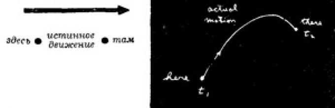
“This is what my teacher Bader told me then: “Let, for example, you have a particle in the gravitational field; this particle, having come out from somewhere, freely moves somewhere else to another point. You threw it, say, up, and it flew up and then fell.

It took her some time to travel from the starting place to the final place. Now try some other movement. Let her move “from here to here” no longer as before, but like this:

But I still found myself in the right place at the same moment in time as before.”

“And so,” the teacher continued, “if you calculate the kinetic energy at each moment of time along the path of the particle, subtract the potential energy from it and integrate the difference over the entire time when the movement occurred, you will see that the number you get will be more, than for true particle motion.

In other words, Newton's laws can be formulated not as F=ma, but as follows: average kinetic energy minus average potential energy reaches its lowest value along the trajectory along which an object actually moves from one place to another.

I'll try to explain this to you a little more clearly.
If we take the gravitational field and designate the trajectory of the particle x(t), Where X- height above the ground (let’s get by with one dimension for now; let the trajectory run only up and down, and not to the sides), then the kinetic energy will be y 2 m(dx/ dt) 2 , a potential energy at an arbitrary moment of time will be equal to mgx.

Now, for some moment of movement along the trajectory, I take the difference between the kinetic and potential energies and integrate over the entire time from beginning to end. Let at the initial moment of time t x the movement began at some height and ended at the moment t 2 at another certain height.

Then the integral is equal to ∫ t2 t1 dt

True motion occurs along a certain curve (as a function of time it is a parabola) and leads to a certain integral value. But you can beforeput imagine some other movement: first a sharp rise, and then some bizarre fluctuations.

You can calculate the difference between potential and kinetic energies on this path... or on any other. And the most amazing thing is that the real path is the one along which this integral is the smallest.
Let's check it out. First, let's look at this case: a free particle has no potential energy at all. Then the rule says that when moving from one point to another in a given time, the integral of the kinetic energy should be the smallest. This means that the particle must move uniformly. (And this is correct, you and I know that the speed in such movement is constant.) Why uniformly? Let's figure it out. If it were otherwise, then at times the speed of the particle would exceed the average, and at times it would be below it, and the average speed would be the same, because the particle would have to get “from here to here” in the agreed upon time. For example, if you need to get from home to school in your car in a certain time, then you can do this in different ways: you can drive like crazy at first and slow down at the end, or drive at the same speed, or you can even go to the opposite side, and only then turn towards the school, etc. In all cases, the average speed, of course, should be the same - the quotient of the distance from home to school divided by time. But even at this average speed, sometimes you moved too fast, and sometimes too slow. And average square something that deviates from the average is, as we know, always larger than the square of the average; This means that the integral of kinetic energy during fluctuations in the speed of movement will always be greater than when moving at a constant speed. You see that the integral will reach a minimum when the speed is constant (in the absence of forces). The right way is this.

An object thrown upward in a field of gravity rises quickly at first, and then more and more slowly. This happens because it also has potential energy, and its minimum value should reach onceness between kinetic and potential energies.. Since potential energy increases as you rise, then less difference It will work if you reach those heights where the potential energy is high as quickly as possible. Then, subtracting this high potential from the kinetic energy, we achieve a decrease in the average. So the path that goes up and supplies a good negative piece at the expense of potential energy is more profitable.

That's all my teacher told me, because he was a very good teacher and knew when it was time to stop. I myself, alas, am not like that. It's hard for me to stop on time. And so, instead of just sparking your interest with my story, I want to intimidate you, I want to make you sick of the complexity of life - I will try to prove what I told you about. The mathematical problem that we will solve is very difficult and unique. There is a certain quantity S, called action. It is equal to kinetic energy minus potential energy integrated over time:

But on the other hand, you can't move too fast or go too high, because that would require too much kinetic energy. You have to move fast enough to get up and down within the given time available to you. So you shouldn't try to fly too high, but just reach some reasonable level. As a result, it turns out that the solution is a kind of balance between the desire to obtain as much potential energy as possible and the desire to reduce the amount of kinetic energy as much as possible - this is the desire to achieve a maximum reduction in the difference between kinetic and potential energies.”

Don't forget that p.e. and k.e.—both functions of time. For any new conceivable path, this action takes on its specific meaning. The mathematical problem is to determine which curve has this number less than the others.

You say, “Oh, this is just a simple example of maximum and minimum. We need to calculate the action, differentiate it and find the minimum.”

But wait. Usually we have a function of some variable and need to find the value variable, at which the function becomes smallest or largest. Let's say there is a rod heated in the middle. Heat spreads over it and its own temperature is established at each point of the rod. You need to find the point where it is highest. But we are talking about something completely different - every path in space answers its number, and is supposed to find that one path, for which this number is minimal. This is a completely different area of mathematics. This is not ordinary calculus, but variational(that's what they call him).

This area of mathematics has many of its own problems. Say, a circle is usually defined as the locus of points whose distances from a given point are the same, but a circle can be defined differently: it is one of the curves given length, which encloses the largest area. Any other curve of the same perimeter encloses an area smaller than the circle. So if we set the task: to find the curve of a given perimeter that bounds the largest area, then we will have a problem from the calculus of variations, and not from the calculus to which you are accustomed.

So, we want to take the integral over the path traveled by the body. Let's do it this way. The whole point is to imagine that there is a true path and that any other curve that we draw is not the real path, so that if we calculate the action for it, we will get a number higher than what we get for the action corresponding to the real way.

So, the task is to find the true path. Where does it lie? One way, of course, would be to count the action for millions and millions of paths and then see which path has the smallest action. This is the path in which the action is minimal and will be real.

This method is quite possible. However, it can be done simpler. If there is a quantity that has a minimum (from ordinary functions, say, temperature), then one of the properties of the minimum is that when moving away from it at a distance first of order of smallness, the function deviates from its minimum value only by the amount second order. And in any other place on the curve, a shift by a small distance changes the value of the function also by a value of the first order of smallness. But at a minimum, slight deviations to the side do not lead to a change in function as a first approximation.

It is this property that we are going to use to calculate the real path.

If the path is correct, then a curve slightly different from it will not lead, as a first approximation, to a change in the magnitude of the action. All changes, if this was truly the minimum, will appear only in the second approximation.

This is easy to prove. If, with some deviation from the curve, changes occur in the first order, then these changes are in effect proportional deviation. They are likely to increase the effect; otherwise it would not be a minimum. But once the changes proportional deviation, then changing the sign of the deviation will reduce the action. It turns out that when you deviate in one direction, the effect increases, and when you deviate in the opposite direction, it decreases. The only possibility for this to really be a minimum is that, as a first approximation, no changes occur and the changes are proportional to the square of the deviation from the actual path.

So, we will go along the following path: denote by x(t) (with a line below) the true path is the one we want to find. Let's take some trial run x(t), differing from the desired one by a small amount, which we denote η (t).

The idea is that if we count the action S on a way x(t), then the difference between this S and by the action that we calculated for the path x(t) (for simplicity it will be designated S), or the difference between S_ And S, should be a first approximation η zero. They can differ in the second order, but in the first the difference must be zero.

And this must be observed for everyone η . However, not quite for everyone. The method requires taking into account only those paths that all begin and end at the same pair of points, i.e., every path must begin at a certain point at the time t 1 and end at another specific point at the moment t 2 . These points and moments are recorded. So our function d) (deviation) must be zero at both ends: η (t 1 )= 0 And η (t 2)=0. Under this condition, our mathematical problem becomes completely defined.

If you didn't know calculus, you could do the same thing to find the minimum of an ordinary function f(x). Would you think about what would happen if you took f(x) and add to X small amount h, and would argue that the amendment to f(x) in first order h should be at a minimum equal to zero. Would you set me up x+h instead of X and would expand j(x+h) up to the first power h. . ., in a word, would repeat everything that we intend to do with η .

If we now look at this carefully, we will see that the first two terms written here correspond to that action S, which I would write for the sought true path X. I want to focus your attention on change. S, i.e. on the difference between S and so S_, which would result for the true path. We will write this difference as bS and let's call it a variation S. Discarding the “second and higher orders”, we obtain for σS

Now the task looks like this. Here in front of me is some integral. I don’t know yet what it’s like, but I know for sure that, what η No matter what, this integral must be equal to zero. “Well,” you might think, “the only way for this to happen is for the multiplier to η was equal to zero." But what about the first term, where there is d η / dt? You say: "If η turns into nothing, then its derivative is the same nothing; this means the coefficient at dv\/ dt must also be zero." Well, that's not entirely true. This is not entirely true because between the deviation η and its derivative there is a connection; they are not completely independent because η (t) must be zero and t 1 and at t 2 .

When solving all problems of the calculus of variations, the same general principle is always used. You slightly shift what you want to vary (similar to what we did by adding η ), glance at the first order terms, then arrange everything so that you get an integral in the following form: “shift (η ), multiplied by what it turns out”, but so that it does not contain any derivatives of η (no d η / dt). It is absolutely necessary to transform everything so that “something” remains, multiplied by η . Now you will understand why this is so important. (There are formulas that will tell you how in some cases you can do this without any calculations; but they are not so general that they are worth memorizing; it is best to do the calculations the way we do it.)

How can I remake a penis d η / dt, so that it appears η ? I can achieve this by integrating piece by piece. It turns out that in the calculus of variations the whole trick is to describe the variation S and then integrate by parts so that the derivatives of η disappeared. In all problems in which derivatives appear, the same trick is performed.

Recall the general principle of integration by parts. If you have an arbitrary function f multiplied by d η / dt and integrated with t, then you write the derivative of η /t

The limits of integration must be substituted into the first term t 1 And t 2 . Then under the integral I will receive the term from integration by parts and the last term that remains unchanged during the transformation.
And now what always happens is happening - the integrated part disappears. (And if it does not disappear, then the principle needs to be reformulated, adding conditions that ensure such disappearance!) We have already said that η at the ends of the path must be equal to zero. After all, what is our principle? The fact is that the action is minimal provided that the varied curve begins and ends at selected points. It means that η (t 1)=0 and η (t 2)=0. Therefore, the integrated term turns out to be zero. We gather the rest of the members together and write

Variation S has now acquired the form that we wanted to give it: something is in brackets (let’s denote it F), and all this is multiplied by η (t) and integrated from t t before t 2 .
It turned out that the integral of some expression multiplied by η (t), always equal to zero:

Is there some function from t; I multiply it by η (t) and integrate it from start to finish. And whatever it is η, I get zero. This means that the function F(t) equal to zero. In general, this is obvious, but just in case, I’ll show you one way to prove it.

Let as η (t) I will choose something that is equal to zero everywhere, for all t, except for one pre-selected value t. It stays zero until I get there t, s Then it jumps for a moment and immediately falls back. If you take the integral of this m) multiplied by some function F, the only place you'll get something non-zero is where η (t) jumped up; and you will get the value F at this point on the integral over the jump. The integral over the jump itself is not equal to zero, but after multiplication by F it should give zero. This means that the function in the place where there was a jump must turn out to be zero. But the leap could have been made anywhere; Means, F must be zero everywhere.

We see that if our integral is equal to zero for any η , then the coefficient at η should go to zero. The action integral reaches a minimum along the path that will satisfy such a complex differential equation:

It's actually not that complicated; you've met him before. It's just F=ma. The first term is mass times acceleration; the second is the derivative of potential energy, i.e. force.

So we have shown (at least for a conservative system) that the principle of least action leads to the correct answer; he states that the path that has the minimum action is the path that satisfies Newton's law.

One more remark needs to be made. I haven't proven this minimum. Maybe this is the maximum. In fact, this does not have to be the minimum. Here everything is the same as in the “shortest time principle”, which we discussed while studying optics. There, too, we first talked about the “shortest” time. However, it turned out that there are situations in which this time is not necessarily the “shortest”. The fundamental principle is that for any first order deviations from the optical path changes in time would be equal to zero; It's the same story here. By "minimum" we actually mean that to the first order of smallness of the change in quantity S when deviations from the path should be equal to zero. And this is not necessarily the “minimum”.

Now I want to move on to some generalizations. First of all, this whole story could be done in three dimensions. Instead of simple X I would then have x, y And z as functions t, and the action would look more complicated. When moving in 3D you must use full kinetic energy): (t/2), multiplied by the square of the total speed. In other words

Additionally, potential energy is now a function x, y And z. What can you say about the path? A path is a certain general curve in space; it is not so easy to draw, but the idea remains the same. What about η? Well, η also has three components. The path can be shifted both in x and in y, and by z, or in all three directions simultaneously. So η now a vector. This does not create any major complications. Only variations must be equal to zero first order then the calculation can be carried out sequentially with three shifts. First you can move ts only in the direction X and say that the coefficient should go to zero. You get one equation. Then we'll move ts in the direction at and we get the second one. Then move in the direction z and we get the third. You can do everything, if you like, in a different order. Be that as it may, a trio of equations arises. But Newton’s law is also three equations in three dimensions, one for each component. You are left to see for yourself that this all works in three dimensions (there is not much work here). By the way, you can take any coordinate system you like, polar, any, and immediately obtain Newton’s laws in relation to this system, considering what happens when a shift occurs η along a radius or along an angle, etc.

The method can be generalized to an arbitrary number of particles. If, say, you have two particles and there are some forces acting between them and there is mutual potential energy, then you simply add their kinetic energies and subtract the interaction potential energy from the sum. What do you vary? Paths both particles. Then for two particles moving in three dimensions, six equations arise. You can vary the position of particle 1 in the direction X, in the direction at and towards z, and do the same with particle 2, so there are six equations. And that's how it should be. Three equations determine the acceleration of particle 1 due to the force acting on it, and the other three determine the acceleration of particle 2 due to the force acting on it. Always follow the same rules of the game and you will get Newton's law for an arbitrary number of particles.

I said we would get Newton's law. This is not entirely true, because Newton's law also includes non-conservative forces, such as friction. Newton argued that that equals any F. The principle of least action is valid only for conservative systems, such where all forces can be obtained from a potential function. But you know that at the microscopic level, that is, at the deepest physical level, non-conservative forces do not exist. Non-conservative forces (such as friction) arise only because we neglect microscopic complex effects: there are simply too many particles to analyze. Fundamental same laws can be expressed as the principle of least action.

Let me move on to further generalizations. Suppose we are interested in what will happen when the particle moves relativistically. So far we have not obtained the correct relativistic equation of motion; F=ma is true only in non-relativistic motions. The question arises: is there a corresponding principle of least action in the relativistic case? Yes, it exists. The formula in the relativistic case is:

The first part of the action integral is the product of the rest mass t 0 on from 2 and to the integral of the speed function √ (1- v 2 /c 2 ). Then, instead of subtracting the potential energy, we have integrals of the scalar potential φ and the vector potential A times v. Of course, only electromagnetic forces are taken into account here. All electric and magnetic fields are expressed in terms of φ and A. This action function gives a complete theory of the relativistic motion of an individual particle in an electromagnetic field.

Of course, you must understand that wherever I wrote v, before making calculations, you should substitute dx/ dt instead of v x etc. Moreover, where I simply wrote x, y, z, you have to imagine the points at the moment t: x(t), y(t), z(t). Actually, only after such substitutions and substitutions of v will you get a formula for the action of a relativistic particle. Let the most skilled among you try to prove that this formula for action actually gives the correct equations of motion for the theory of relativity. Let me just advise you to start by discarding A, that is, do without magnetic fields for now. Then you will have to obtain the components of the equation of motion dp/dt=—qVφ, where, as you probably remember, p=mv√(1-v 2 /c 2).

It is much more difficult to include the vector potential A into consideration. The variations then become incomparably more complex. But in the end the force turns out to be equal to what it should be: g(E+v × B). But have some fun with it yourself.

I would like to emphasize that in the general case (for example, in the relativistic formula), the integral in action no longer includes the difference between kinetic and potential energies. This was only suitable in a non-relativistic approximation. For example, member m o c 2√(1-v 2 /c 2)-This is not what is called kinetic energy. The question of what the action should be for any particular case can be decided after some trial and error. This is the same type of problem as determining what the equations of motion should be. You just have to play with the equations you know and see if they can be written as the principle of least action.

One more note about terminology. That function that is integrated over time to obtain an action S, called LagrangianΛ. This is a function that depends only on the velocities and positions of the particles. So the principle of least action is also written in the form

where under X i And v i all components of coordinates and velocities are implied. If you ever hear someone talk about the "Lagrangian", they are talking about the function used to obtain S. For relativistic motion in an electromagnetic field

In addition, I should note that the most meticulous and pedantic people do not call S action. It is called "Hamilton's first principal function". But giving a lecture on “Hamilton's principle of least first principal function” was beyond my strength. I called it "action". And besides, more and more people call it “action.” You see, historically action has been called something else that is not as useful to science, but I think it makes more sense to change the definition. Now you too will begin to call the new function an action, and soon everyone will begin to call it by this simple name.

Now I want to tell you something about our topic that is similar to the reasoning that I had about the principle of the shortest time. There is a difference in the very essence of the law that says that some integral taken from one point to another has a minimum - the law that tells us something about the whole path at once, and the law that says that when you move, then This means there is a force leading to acceleration. The second approach reports to you about your every step, it traces your path inch by inch, and the first immediately gives some general statement about the entire path traveled. While talking about light, we talked about the connection between these two approaches. Now I want to explain to you why differential laws should exist if there is such a principle - the principle of least action. The reason is this: let us consider the path actually traveled in space and time. As before, we will make do with one measurement, so that we can draw a graph of the dependence X from t. Along the true path S reaches a minimum. Let's assume that we have this path and that it passes through some point A space and time and through another neighboring point b.

Now, if the entire integral of t 1 before t 2 has reached a minimum, it is necessary that the integral along a small section from a to b was also minimal. It can't be that part of A before b at least a little more than the minimum. Otherwise, you could move the curve back and forth in this section and slightly reduce the value of the entire integral.

This means that any part of the path should also provide a minimum. And this is true for any small portions of the path. Therefore, the principle that the entire path should give a minimum can be formulated by saying that an infinitesimal segment of the path is also a curve on which the action is minimal. And if we take a short enough segment of the path - between points very close to each other A And b,- then it doesn’t matter how the potential changes from point to point far from this place, because, going through your entire short segment, you almost never move from that place. The only thing you need to consider is the first order change in smallness in the potential. The answer may depend only on the derivative of the potential, and not on the potential elsewhere. Thus, a statement about the property of the entire path as a whole becomes a statement about what happens on a short section of the path, i.e., a differential statement. And this differential formulation includes derivatives of the potential, that is, the force at a given point. This is a qualitative explanation of the connection between the law as a whole and the differential law.

When we talked about light, we also discussed the question: how does a particle find the right path? From a differential point of view, this is easy to understand. At every moment the particle experiences acceleration and knows only what it is supposed to do at that moment. But all your instincts of cause and effect rear up when you hear that a particle “decides” which path to take, striving for a minimum of action. Isn’t she “sniffing” the neighboring paths, figuring out what they will lead to - more or less action? When we placed a screen in the path of light so that the photons could not try all the paths, we found out that they could not decide which path to take, and we got the phenomenon of diffraction.

But is this also true for mechanics? Is it true that a particle not only “goes the right way”, but reconsiders all other conceivable trajectories? And what if, by putting obstacles in its path, we do not allow it to look ahead, then we will get some kind of analogue of the phenomenon of diffraction? The most wonderful thing about all this is that everything really is like this. This is exactly what the laws of quantum mechanics say. So our principle of least action is not fully formulated. It does not consist in the fact that the particle chooses the path of least action, but in the fact that it “senses” all neighboring paths and chooses the one along which the action is minimal, and the method of this choice is similar to the way in which light selects the shortest time. You remember that the way light selects the shortest time is this: if light goes along a path that requires a different time, it will arrive with a different phase. And the total amplitude at some point is the sum of the amplitude contributions for all the paths along which light can reach it. All those paths whose phases differ sharply do not yield anything after addition. But if you managed to find the entire sequence of paths, the phases of which are almost the same, then the small contributions will add up, and at the arrival point the total amplitude will receive a noticeable value. The most important path is the one near which there are many close paths that give the same phase.

Exactly the same thing happens in quantum mechanics. Complete quantum mechanics (non-relativistic and neglecting electron spin) works like this: the probability that a particle leaving a point 1 in the moment t 1, will reach the point 2 in the moment t 2 , equal to the square of the probability amplitude. The total amplitude can be written as the sum of the amplitudes for all possible paths—for any arrival path. For anyone x(t), which could occur for any conceivable imaginary trajectory, the amplitude must be calculated. Then they all need to be folded. What do we take as the probability amplitude of a certain path? Our action integral tells us what the amplitude of an individual path should be. Amplitude is proportional e tS/h, Where S - action along this path. This means that if we represent the phase of the amplitude as a complex number, then the phase angle will be equal to S/ h. Action S has the dimension of energy over time, and Planck's constant has the same dimension. This is the constant that determines when quantum mechanics is needed.

And that's how it all works. Let action for all paths S will be very large compared to the number h. Let some path lead to a certain amplitude value. The phase of the adjacent path will be completely different, because with a huge S even minor changes S abruptly change phase (after all h extremely little). This means that adjacent paths usually extinguish their contributions when added. And only in one area is this not true - in the one where both the path and its neighbor - both, to a first approximation, have the same phase (or, more precisely, almost the same action, varying within h). Only such paths are taken into account. And in the limiting case, when Planck’s constant h tends to zero, the correct quantum mechanical laws can be summarized by saying: “Forget about all those probability amplitudes. The particle actually moves along a special path - exactly the one along which S to a first approximation does not change.” This is the connection between the principle of least action and quantum mechanics. The fact that quantum mechanics can be formulated in this way was discovered in 1942 by a student of the same teacher, Mr. Bader, whom I told you about. [Quantum mechanics was originally formulated using a differential equation for amplitude (Schrödinger) as well as some matrix mathematics (Heisenberg).]

Now I want to talk about other principles of minimum in physics. There are many interesting principles of this kind. I will not list them all, but I will name only one more. Later, when we get to one physical phenomenon for which there is an excellent minimum principle, I will tell you about it. Now I want to show that it is not necessary to describe electrostatics using a differential equation for the field; one can instead require that some integral have a maximum or a minimum. To begin with, let's take the case when the charge density is known everywhere, but we need to find the potential φ at any point in space. You already know that the answer should be:

Another way to say the same thing is to evaluate the integral U*

this is a volume integral. It is taken throughout the space. With correct potential distribution φ (x, y,z) this expression reaches its minimum.

We can show that both of these statements regarding electrostatics are equivalent. Let's assume that we have chosen an arbitrary function φ. We want to show that when we take as φ the correct value of the potential _φ plus a small deviation f, then to the first order of smallness the change in U* will be equal to zero. So we write

here φ is what we are looking for; but we will vary φ to see what it must be in order for the variation U* turned out to be of the first order of smallness. In the first term U* we need to write

This needs to be integrated by x, y and by z. And here the same trick suggests itself: in order to get rid of df/ dx, we will integrate over X in parts. This will lead to additional differentiationφ with respect to X. This is the same basic idea with which we got rid of derivatives with respect to t. We use equality

The integrated term is zero because we take f to be zero at infinity. (This corresponds to η vanishing as t 1 And t 2 . So our principle is more precisely formulated as follows: U* for the right φ less than for any other φ(x, y,z), having the same values at infinity.) Then we will do the same with at and with z. Our integral ΔU* will turn into

For this variation to be equal to zero for any arbitrary f, the coefficient of f must be equal to zero. Means,

We're back to our old equation. This means that our “minimum” proposal is correct. It can be generalized if the calculations are slightly modified. Let's go back and integrate part by part, without describing everything component by component. Let's start by writing the following equality:

By differentiating the left side, I can show that it is exactly equal to the right. This equation is suitable for performing integration by parts. In our integral ΔU* we replace Vφ*Vf n and fV 2 φ+V*(fVφ) and then integrate this over the volume. The divergence term after integration over the volume is replaced by an integral over the surface:

And since we integrate over the entire space, the surface in this integral lies at infinity. This means f=0, and we get the same result.

Only now are we beginning to understand how to solve problems in which we we don't know where all the charges are located. Let us have conductors on which charges are somehow distributed. If the potentials on all conductors are fixed, then our minimum principle is still allowed to apply. Integration into U* we will draw only along the area lying outside all the conductors. But since we cannot change (φ) on conductors, then on their surface f = 0, and the surface integral

need to be done only in the spaces between the conductors. And we, of course, get the Poisson equation again

We have therefore shown that our original integral U* reaches a minimum even when it is calculated in the space between conductors, each of which is at a fixed potential [this means that each test function φ(g, y,z) must be equal to the specified conductor potential when (x, y,z) - points of the conductor surface]. There is an interesting special case when charges are located only on conductors. Then

and our minimum principle tells us that in the case where each conductor has its own predetermined potential, the potentials in the spaces between them are adjusted so that the integral U* turns out to be as small as possible. What kind of integral is this? The term Vφ is the electric field. This means that the integral is electrostatic energy. The correct field is the only one that, of all the fields obtained as a potential gradient, has the lowest total energy.

I would like to use this result to solve some particular problem and show you that all these things have real practical significance. Suppose I took two conductors in the form of a cylindrical capacitor.

The inner conductor has a potential equal to, say, V, and for the external one - zero. Let the radius of the inner conductor be equal to A, and external - b. Now we can assume that the distribution of potentials between them is any. But if we take correct value of φ and calculate
(ε 0 /2) ∫ (Vφ) 2 dV then the energy of the system should be 1/2CV 2.

So using our principle you can calculate the capacity WITH. If we take an incorrect potential distribution and try to estimate the capacitance of the capacitor using this method, we will arrive at an overly large capacitance value for a fixed V. Any estimated potential φ that does not exactly coincide with its true value will also lead to an incorrect value of C, greater than necessary. But if the incorrectly chosen potential cp is still a rough approximation, then the capacitance WITH will turn out with good accuracy, because the error in C is a second order value compared to the error in φ.

Let's assume that I don't know the capacitance of the cylindrical capacitor. Then, to recognize her, I can use this principle. I will simply test different functions of φ as a potential until I achieve the lowest value WITH. Let's say, for example, that I have chosen a potential that corresponds to a constant field. (You know, of course, that the field here is not actually constant; it varies as 1/r) If the field is constant, this means that the potential depends linearly on distance. In order for the voltage on the conductors to be as required, the function φ must have the form

This function is equal to V at r=a, zero at r =b, and between them there is a constant slope equal to - V/(b—A). So, to determine the integral U*, you just need to multiply the square of this gradient by ε o /2 and integrate over the entire volume. Let us carry out this calculation for a cylinder of unit length. Volume element at radius r equals 2πrdr. Carrying out the integration, I find that my first test gives the following capacity:

So I get a formula for capacity, which, although incorrect, is some kind of approximation:

Of course it's different from the correct answer C=2πε 0 /ln (b/a), but overall it's not that bad. Let's try to compare it with the correct answer for several values b/a. The numbers I calculated are shown in the following table.

Even when b/a=2(and this already leads to quite large differences between the constant and linear fields), I still get a fairly passable approximation. The answer, of course, as expected, is a little too high. But if a thin wire is placed inside a large cylinder, then everything looks much worse. Then the field changes very much and replacing it with a constant field does not lead to anything good. When b/a = 100, we overestimate the answer by almost twice. For small ones b/a the situation looks much better. In the opposite limit, when the gap between the conductors is not very wide (say, for b/a = 1.1), a constant field turns out to be a very good approximation, it gives the value WITH accurate to tenths of a percent.

Now I will tell you how to improve this calculation. (The answer for the cylinder is, of course, famous, but the same method works for some other unusual capacitor shapes for which you may not know the correct answer.) The next step is to find a better approximation for the unknown true potential φ. Let's say you can test the constant plus the exponent φ, etc. But how do you know you've got the best approximation if you don't know the true φ? Answer: Count it up WITH; the lower it is, the closer to the truth. Let's test this idea. Let the potential be not linear, but, say, quadratic in r, and the electric field not constant, but linear. The most general quadratic form, which turns into φ=O when r=b and in φ=F at r=a, is this:

where α is a constant number. This formula is a little more complicated than the previous one. It includes both a quadratic term and a linear one. It is very easy to get a field from it. It's equal to simple

Now this needs to be squared and integrated over the volume. But wait a minute. What should I take for α? I can take f to be a parabola, but which one? Here's what I'll do: calculate the capacity at arbitrary α. I will get

This looks a little confusing, but that’s how it turns out after integrating the square of the field. Now I can choose for myself. I know the truth lies lower than anything I'm about to calculate. No matter what I put in place of a, the answer will still be too big. But if I continue my game with α and try to achieve the lowest possible value WITH, then this lowest value will be closer to the truth than any other value. Therefore, I now need to choose α so that the value WITH has reached its minimum. Turning to ordinary differential calculus, I am convinced that the minimum WITH will be when α =— 2 b/(b+a). Substituting this value into the formula, I get for the smallest capacity

I figured out what this formula gives for WITH at different values b/a. I named these numbers WITH(quadratic). Here is a table that compares WITH(quadratic) with WITH(true).

For example, when the radius ratio is 2:1, I get 1.444. This is a very good approximation to the correct answer, 1.4423. Even with large Ya the approximation remains quite good—much better than the first approximation. It remains tolerable (overestimated by only 10%) even with b/a = 10: 1. A large discrepancy occurs only at a ratio of 100: 1. I get WITH equal to 0.346 instead of 0.267. On the other hand, for a radius ratio of 1.5 the agreement is excellent, and for b/a=1.1 the answer is 10.492065 instead of the expected 10.492070. Where you would expect a good answer, it turns out to be very, very good.

I have given all these examples, firstly, to demonstrate the theoretical value of the principle of minimal action and in general of all principles of minimum, and, secondly, to show you their practical usefulness, and not at all in order to calculate the capacity that we already have we know very well. For any other shape, you can try an approximate field with a few unknown parameters (like α) and fit them to the minimum. You will obtain superior numerical results on problems that cannot be solved otherwise.

They obey it, and therefore this principle is one of the key provisions of modern physics. The equations of motion obtained with its help are called the Euler-Lagrange equations.

The first formulation of the principle was given by P. Maupertuis in the year, immediately pointing out its universal nature, considering it applicable to optics and mechanics. From this principle he derived the laws of reflection and refraction of light.

Story

Maupertuis came to this principle from the feeling that the perfection of the Universe requires a certain economy in nature and contradicts any useless expenditure of energy. The natural movement must be such as to make a certain quantity minimum. All he had to do was find this value, which he continued to do. It was the product of the duration (time) of movement within the system by twice the value, which we now call the kinetic energy of the system.

Euler (in "Réflexions sur quelques loix générales de la nature", 1748) adopts the principle of least amount of action, calling action "effort". Its expression in statics corresponds to what we would now call potential energy, so that its statement of least action in statics is equivalent to the minimum potential energy condition for an equilibrium configuration.

In classical mechanics

The principle of least action serves as the fundamental and standard basis of the Lagrangian and Hamiltonian formulations of mechanics.

First let's look at the construction like this: Lagrangian mechanics. Using the example of a physical system with one degree of freedom, let us recall that an action is a functional with respect to (generalized) coordinates (in the case of one degree of freedom - one coordinate), that is, it is expressed through such that each conceivable version of the function is associated with a certain number - an action (in In this sense, we can say that an action as a functional is a rule that allows for any given function to calculate a well-defined number - also called an action). The action looks like:

where is the Lagrangian of the system, depending on the generalized coordinate, its first derivative with respect to time, and also, possibly, explicitly on time. If the system has a larger number of degrees of freedom, then the Lagrangian depends on a larger number of generalized coordinates and their first derivatives with respect to time. Thus, the action is a scalar functional depending on the trajectory of the body.

The fact that the action is a scalar makes it easy to write it in any generalized coordinates, the main thing is that the position (configuration) of the system is unambiguously characterized by them (for example, instead of Cartesian coordinates, these can be polar coordinates, distances between points of the system, angles or their functions, etc. .d.).

The action can be calculated for a completely arbitrary trajectory, no matter how “wild” and “unnatural” it may be. However, in classical mechanics, among the entire set of possible trajectories, there is only one along which the body will actually go. The principle of stationary action precisely gives the answer to the question of how the body will actually move:

This means that if the Lagrangian of the system is given, then using the calculus of variations we can establish exactly how the body will move by first obtaining the equations of motion - the Euler-Lagrange equations, and then solving them. This allows not only to seriously generalize the formulation of mechanics, but also to choose the most convenient coordinates for each specific problem, not limited to Cartesian ones, which can be very useful for obtaining the simplest and most easily solved equations.

where is the Hamilton function of this system; - (generalized) coordinates, - conjugate (generalized) impulses, which together characterize at each given moment of time the dynamic state of the system and, each being a function of time, thus characterizing the evolution (motion) of the system. In this case, to obtain the equations of motion of the system in the form of Hamilton’s canonical equations, it is necessary to vary the action written in this way independently for all and .

It should be noted that if from the conditions of the problem it is possible in principle to find the law of motion, then this is automatically Not means that it is possible to construct a functional that takes a stationary value during true motion. An example is the joint movement of electric charges and monopoles - magnetic charges - in an electromagnetic field. Their equations of motion cannot be derived from the principle of stationary action. Likewise, some Hamiltonian systems have equations of motion that cannot be derived from this principle.

Examples

Trivial examples help to evaluate the use of the operating principle through the Euler-Lagrange equations. Free particle (mass m and speed v) in Euclidean space moves in a straight line. Using the Euler-Lagrange equations, this can be shown in polar coordinates as follows. In the absence of potential, the Lagrange function is simply equal to the kinetic energy

in an orthogonal coordinate system.

In polar coordinates, the kinetic energy, and hence the Lagrange function, becomes

The radial and angular components of the equations become, respectively:

Solving these two equations

Here is a conditional notation for infinitely multiple functional integration over all trajectories x(t), and is Planck’s constant. We emphasize that, in principle, the action in the exponential appears (or can appear) itself when studying the evolution operator in quantum mechanics, but for systems that have an exact classical (non-quantum) analogue, it is exactly equal to the usual classical action.

Mathematical analysis of this expression in the classical limit - for sufficiently large , that is, for very fast oscillations of the imaginary exponential - shows that the overwhelming majority of all possible trajectories in this integral cancel each other in the limit (formally for ). For almost any path there is a path on which the phase shift will be exactly the opposite, and they will add up to zero contribution. Only those trajectories for which the action is close to the extreme value (for most systems - to the minimum) are not reduced. This is a purely mathematical fact from the theory of functions of a complex variable; For example, the stationary phase method is based on it.

As a result, the particle, in full agreement with the laws of quantum mechanics, moves simultaneously along all trajectories, but under normal conditions only trajectories close to stationary (that is, classical) contribute to the observed values. Since quantum mechanics transforms into classical mechanics in the limit of high energies, we can assume that this is quantum mechanical derivation of the classical principle of stationarity of action.

In quantum field theory

In quantum field theory, the principle of stationary action is also successfully applied. The Lagrangian density here includes the operators of the corresponding quantum fields. Although it is more correct here in essence (with the exception of the classical limit and partly quasi-classics) to speak not about the principle of stationarity of action, but about Feynman integration along trajectories in the configuration or phase space of these fields - using the just mentioned Lagrangian density.

Further generalizations

More broadly, an action is understood as a functional that defines a mapping from a configuration space to a set of real numbers and, in general, it does not have to be an integral, because non-local actions are possible in principle, at least theoretically. Moreover, a configuration space is not necessarily a function space because it can have non-commutative geometry.

They obey it, and therefore this principle is one of the key provisions of modern physics. The equations of motion obtained with its help are called the Euler-Lagrange equations.

Story

In classical mechanics

The principle of least action serves as the fundamental and standard basis of the Lagrangian and Hamiltonian formulations of mechanics.

Examples

in an orthogonal coordinate system.

In polar coordinates, the kinetic energy, and hence the Lagrange function, becomes

The radial and angular components of the equations become, respectively:

Solving these two equations

In quantum field theory

Further generalizations

The principle of least action, first formulated precisely by Jacobi, is similar to Hamilton's principle, but less general and more difficult to prove. This principle is applicable only to the case when the connections and force function do not depend on time and when, therefore, there is an integral of living force.

This integral has the form:

Hamilton's principle stated above states that the variation of the integral

is equal to zero upon the transition of the actual motion to any other infinitely close motion, which transfers the system from the same initial position to the same final position in the same period of time.

Jacobi's principle, on the contrary, expresses a property of motion that does not depend on time. Jacobi considers the integral

determining action. The principle he established states that the variation of this integral is zero when we compare the actual motion of the system with any other infinitely close motion that takes the system from the same initial position to the same final position. In this case, we do not pay attention to the time period spent, but we observe equation (1), i.e., the equation of manpower with the same value of the constant h as in actual movement.

This necessary condition for an extremum leads, generally speaking, to a minimum of integral (2), hence the name principle of least action. The minimum condition seems to be the most natural, since the value of T is essentially positive, and therefore integral (2) must necessarily have a minimum. The existence of a minimum can be strictly proven if only the time period is small enough. The proof of this position can be found in Darboux's famous course on surface theory. We, however, will not present it here and will limit ourselves to deriving the condition

432. Proof of the principle of least action.

In the actual calculation we encounter one difficulty that is not present in the proof of Hamilton's theorem. The variable t no longer remains independent of variation; therefore variations of q i and q. are related to the variation of t by a complex relationship that follows from equation (1). The simplest way to get around this difficulty is to change the independent variable, choosing one whose values fall between constant limits that do not depend on time. Let k be a new independent variable, the limits of which are assumed to be independent of t. When moving the system, the parameters and t will be functions of this variable

Let letters with primes q denote derivatives of parameters q with respect to time.

Since the connections, by assumption, do not depend on time, the Cartesian coordinates x, y, z are functions of q that do not contain time. Therefore, their derivatives will be linear homogeneous functions of q and 7 will be a homogeneous quadratic form of q, the coefficients of which are functions of q. We have

To distinguish the derivatives of q with respect to time, we denote, using parentheses, (q), the derivatives of q taken with respect to and put in accordance with this

then we will have

and integral (2), expressed through the new independent variable A, will take the form;

The derivative can be eliminated using the living force theorem. Indeed, the integral of manpower will be

Substituting this expression into the formula for, we reduce integral (2) to the form

The integral defining the action thus took its final form (3). The integrand function is the square root of the quadratic form of the quantities

Let us show that the differential equations of the extremals of the integral (3) are exactly the Lagrange equations. The equations of extremals, based on the general formulas of the calculus of variations, will be:

Let's multiply the equations by 2 and perform partial differentiations, taking into account that it does not contain, then we get, if we do not write an index,

These are equations of extremals expressed in terms of the independent variable. The task now is to return to the independent variable

Since Γ is a homogeneous function of the second degree of and is a homogeneous function of the first degree, we have

On the other hand, the living force theorem can be applied to the factors of derivatives in the equations of extremals, which leads, as we saw above, to the substitution

As a result of all substitutions, the equations of extremals are reduced to the form

We have thus arrived at the Lagrange equations.

433. The case when there are no driving forces.

In the case when there are no driving forces, there is an equation for living force and we have

The condition for the integral to be a minimum is in this case that the corresponding value of -10 must be the smallest. Thus, when there are no driving forces, then among all the movements in which the living force maintains the same given value, the actual movement is that which transfers the system from its initial position to its final position in the shortest time.

If the system is reduced to one point moving on a stationary surface, then the actual movement, among all movements on the surface, performed at the same speed, is the movement in which the point moves from its initial position to the final position in the shortest

time interval. In other words, a point describes on the surface the shortest line between its two positions, i.e., a geodesic line.

434. Note.

The principle of least action assumes that the system has several degrees of freedom, since if there were only one degree of freedom, then one equation would be sufficient to determine the motion. Since the movement can in this case be completely determined by the equation of living force, then the actual movement will be the only one that satisfies this equation, and therefore cannot be compared with any other movement.

LEAST EFFECTIVE PRINCIPLE

One of the variational principles of mechanics, according to Krom, for a given class of mechanical movements compared with each other. system, the valid one is that for which physical. size, called action, has the smallest (more precisely, stationary) value. Usually N. d. p. is used in one of two forms.

a) N. d. p. in the form of Hamilton - Ostrogradsky establishes that among all kinematically possible movements of a system from one configuration to another (close to the first), accomplished in the same period of time, the valid one is the one for which the Hamiltonian action S will be the smallest. Math. the expression of the N. d.p. in this case has the form: dS = 0, where d is the symbol of incomplete (isochronous) variation (i.e., unlike complete variation, time does not vary in it).

b) N. d. p. in the form of Maupertuis - Lagrange establishes that among all kinematically possible movements of a system from one configuration to another close to it, performed while maintaining the same value of the total energy of the system, the valid one is that for - Therefore, the Lagrange action W will be the smallest. Math. the expression of the N. d.p. in this case has the form DW = 0, where D is the symbol of total variation (unlike the Hamilton-Ostrogradsky principle, here not only the coordinates and velocities vary, but also the time of movement of the system from one configuration to another) . N.d.p.v. In this case, it is valid only for conservative and, moreover, holonomic systems, while in the first case, the non-conservative principle is more general and, in particular, can be extended to non-conservative systems. N.D.P. are used to compile equations of mechanical motion. systems and to study the general properties of these movements. With an appropriate generalization of concepts, the NDP finds applications in the mechanics of a continuous medium, in electrodynamics, and quantum. mechanics, etc.

- the same as...
Physical encyclopedia
- m-operator, minimization operator, - a method of constructing new functions from other functions, consisting of the following...
Mathematical Encyclopedia
- one of the variational principles of mechanics, according to which for a given class of mechanical movements compared with each other. system is carried out that for which the action is minimal...
Natural science. encyclopedic Dictionary
- one of the most important laws of mechanics, established by the Russian scientist M.V. Ostrogradsky...
Russian Encyclopedia
Dictionary of legal terms
- in the constitutional law of a number of states the principle according to which generally recognized principles and norms of international law are an integral part of the legal system of the corresponding country...
Encyclopedia of Lawyer
- in the constitutional law of a number of states the principle according to which generally recognized norms of international law are an integral part of the national legal system...
Large legal dictionary
- the shortest distance from the center of the explosive charge to the free surface - line on nai-malkoto resistance - křivka nejmenšího odporu - Line der geringsten Festigkeit - robbantás minimális ellenállási tengelyvonala - hamgiin baga...
Construction dictionary
- if it is possible to move points of a deformable body in different directions, each point of this body moves in the direction of least resistance...
Encyclopedic Dictionary of Metallurgy
- a rule by which existing inventories are usually valued either at the lowest cost or at the lowest selling price...
Dictionary of business terms
- in the constitutional law of a number of states - the principle according to which generally recognized principles and norms of international law are an integral part of the legal system of the relevant state and operate...
Encyclopedic Dictionary of Economics and Law
- one of the variational principles of mechanics, according to which for a given class of movements of a mechanical system compared with each other, the valid one is the one for which the physical quantity,...
- the same as Gauss's principle...
Great Soviet Encyclopedia
- one of the variational principles of mechanics; the same as the principle of least action...
Great Soviet Encyclopedia
- one of the variational principles of mechanics, according to which for a given class of movements of a mechanical system compared with each other, the one for which the action is minimal...
Large encyclopedic dictionary
- Book Choose the easiest method of action, avoiding obstacles, avoiding difficulties...
Phraseological Dictionary of the Russian Literary Language

"THE LEAST VALUE PRINCIPLE" in books

2.5.1. Operating principle of the device

From the book Entertaining Electronics [Unconventional encyclopedia of useful circuits] author Kashkarov Andrey Petrovich

2.5.1. The principle of operation of the device The principle of operation of the device is simple. When the luminous flux emitted by the HL1 LED is reflected from the object and hits the photodetector, the electronic unit, implemented on 2 microcircuits - the KR1401SA1 comparator and the KR1006VI1 timer, produces

The principle of operation of teraphim

From the book Secret Knowledge. Theory and practice of Agni Yoga author Roerich Elena Ivanovna

The principle of operation of teraphim 02.24.39 You know that every awareness and representation of any object thereby brings us closer to it. As you know, the psychic layers of an object can be transferred to its teraphim. The astral teraphim of distant worlds and

Three Conditions for the Law of Least Effort to Apply

From the book The Wisdom of Deepak Chopra [Get what you want by following the 7 laws of the Universe] by Tim Goodman

Three conditions for the Law of Least Effort to operate Let's see what conditions are required to attract this creative flow of energy from the Universe into your life - the energy of love, and therefore for the Law of Least Effort to begin to work in your life.

Chapter 19 PRINCIPLE OF Least EFFECT

From book 6. Electrodynamics author Feynman Richard Phillips

Chapter 19 THE PRINCIPLE OF Least EFFECT Addition made after a lecture When I was at school, our physics teacher, named Bader, once called me in after class and said: “You look as if you are terribly tired of everything; listen to one interesting thing

5. Principle of least action

From the book Revolution in Physics by de Broglie Louis

5. Principle of least action The equations for the dynamics of a material point in a field of forces with potential can be obtained based on the principle, which in general terms is called Hamilton’s principle, or the principle of stationary action. According to this principle, of all

Operating principle

From the book Locksmith's Guide to Locks by Phillips Bill

Principle of operation The ability to rotate the cylinder depends on the position of the pins, which in turn is determined by gravity, the action of springs and the force of the key (or master key; for information on master keys, see Chapter 9). In the absence of a key, gravity and springs press in

Stationary action principle

From the book Great Soviet Encyclopedia (ST) by the author TSB

Principle of least action

TSB

Principle of least coercion

From the book Great Soviet Encyclopedia (NA) by the author TSB

2.5.1. Operating principle

From the book Relay protection in electrical distribution networks B90 author Bulychev Alexander Vitalievich

2.5.1. Operating principle In electrical networks with two-way power supply and in ring networks, conventional current protection cannot operate selectively. For example, in an electrical network with two power sources (Fig. 2.15), where switches and protections are installed on both sides

Operating principle

From the book Turbo Suslik. How to stop fucking yourself up and start living author Leushkin Dmitry

The principle of action “Process this” is, in fact, a kind of “macro” that, with one phrase, launches a whole bunch of processes in the subconscious, the purpose of which is to process the selected mental material. This handler itself includes 7 different modules, some of which

How to Start Following the Law of Least Effort: Three Necessary Actions

From the book A Guide to Growing Capital from Joseph Murphy, Dale Carnegie, Eckhart Tolle, Deepak Chopra, Barbara Sher, Neil Walsh author Stern Valentin

How to start following the Law of Least Effort: three necessary actions For the Law of Least Effort to start working, you must not only comply with the three conditions mentioned above, but also perform three actions. First action: start accepting the world as it is Accept

11. Physics and Aikido of the least action

author Mindell Arnold

11. Physics and Aikido of the smallest effect When it blows, there is only wind. When it rains, there is only rain. When the clouds pass, the sun shines through them. If you open yourself to insight, then you are at one with the insight. And you can use it completely. If you open up

Leibniz's principle of least action "Vis Viva"

From the book Geopsychology in Shamanism, Physics and Taoism author Mindell Arnold

Leibniz's Principle of Least Action "Vis Viva" We all have Wilhelm Gottfried Leibniz (1646–1716) to thank for the principle of least action. One of the first "modern" physicists and mathematicians, Leibniz lived in the time of Newton - an era when scientists were more openly

Aikido - the embodiment of the principle of least action

From the book Geopsychology in Shamanism, Physics and Taoism author Mindell Arnold

Aikido - the embodiment of the principle of least action Our psychology and technology are largely driven by a concept very close to the idea of least action. We are constantly trying to make our lives easier. Today's computers are not fast enough; They have to